《1.Introduction》

1.Introduction

Upstream operations are quite cumbersome to characterize with first-principles models, since they involve different phases and interacting physical phenomena. One of their main tasks is to separate water and oil, which are both extracted from an oil well, in order to send oil to the stabilization, mid-stream, and downstream processes.

Water removal from crude oil has become an area of increasing interest in the last two decades, especially regarding the possibility of exploiting oil deposits that have been disposed of. In fact, it is known that oil deposits still contain a large amount of oil (up to 40% of the initial quantity) when they are disposed of, but the remaining quantity of oil is too spoiled with water (up to the extraction of oily waters), preventing further operations from being economically sustainable.

Nevertheless, the increase in global energy requirements and the increasingly remote locations of new oil deposits are strongly pushing forward the exploitation of disposed plants, with the main issue being that of separating oil and water. Such a separation is usually carried out in a series of operations with long residence times in order to exploit the gap between the densities of oil and water. After these operations, it is necessary to refine the separation in order to remove the remaining portion of water in the oil, which is typically an emulsion of small droplets that cannot be separated by gravity. This quantity of water is not negligible (making up several percent in volume) and can significantly influence the downstream operations of oil stabilization if it is not removed properly.

Moreover, a certain quantity of water is usually added to oil during the oil-well extraction, with the intent of dissolving salts and removing the water-salt solution from the oil before the traditional operations of oil stabilization. As a result, whenever oil is extracted, a certain quantity of water is present in the oil and must be removed.

It is necessary to favor the coalescence of small droplets of the water-oil emulsion in order to obtain larger water droplets that can be separated by gravity. The best industrial practice is to adopt an electrical  field  with  alternate  current  to  continuously  deform  the droplets and try to improve their collisions in the emulsion, in order to progressively increase the average diameter of the water droplets. Such an upstream unit is called an electrostatic coalescer.

The electrostatic coalescer is already well established in oil and gas processes; however, the physical phenomena that govern its behavior are not yet completely understood. It is not a coincidence that the electrostatic coalescer is usually an oversized unit with respect to the rest of the plant. In fact, this overdesign is a way to overcome the current lack of knowledge.

This study is aimed at providing a first-principle mathematical model of an electrostatic coalescer unit, starting from fundamental laws and the existing literature. The mathematical model  can  be used for both design and control purposes in terms of monitoring, prediction, predictive control, and optimization. Section 2 provides the scientific and technological state of the art. Section 3 details the mathematical modeling, starting from the fundamental laws. Section 4 provides a selection of numerical solutions. Section 5 gives the results and provides a sensitivity analysis. Finally, Section 6 provides the conclusions.

《2.State of the art》

2.State of the art

Many experimental and theoretical studies have been proposed to investigate the behavior of electrostatic coalescer units. Those research activities were and are mainly focused on the characterization of the water-oil emulsion, the distribution of the diameters of the water droplets, the effects of the introduction of chemicals and additives to favor coalescence, the effect of the electrical field on the droplets, and the effect of the temperature. A comprehensive technical review has been published by Eow and Ghadiri [1].

《2.1. Water-in-oil emulsion》

2.1. Water-in-oil emulsion

Neglecting the gas phase, which is not of interest for the present study, the electrostatic coalescer is characterized by a biphasic emulsion of water in oil. The emulsion is a mixture of at least two immiscible phases, where the dispersed phase assumes the form of many droplets within the continuous phase [2]. The formation of water-in-oil emulsions originates from the contact between oil and water; although such emulsions usually occur directly in an oil deposit, desalting operations require the introduction of additional water to remove salt by generating an emulsion.

Oil-and-water emulsions can be water dispersed in oil, oil dispersed in water, or multiple conditions such as oil-water-oil. These conditions can be inverted according to the volumetric composition of the dispersed phase. The emulsion of interest in this study is a certain percent in volume of water dispersed in oil. Specifically, we investigate the stability of such an emulsion, meaning the resistance against separating the dispersed phase from the continuous one, in order to determine how to favor the separation of oil and water. Some experiments have demonstrated that a water-oil emulsion can become unstable after passing through valves, pipelines, and certain unit operations; however, other important parameters must be considered in order to better realize a water-in-oil emulsion system and the typical unit operation that is used to separate the phases: the electrostatic coalescer.

A common way to classify an emulsion is related to the droplet diameters in the dispersed phase:

(1)Macro-emulsions. The diameter of the droplets is larger than 0.1 µm. Macro-emulsions are thermodynamically  unstable and the phases can be separated using gravity, albeit with a long operational time. Gravity units can benefit from other contributions such as electrical fields, centrifugation, and so forth, to shorten the operational time. Most oily emulsions belong to this family.

(2)Micro-emulsions. The diameter of the droplets is larger than 10 nm. Micro-emulsions are characterized by a high thermodynamic stability, and their separation is quite complicated.

The stability of an emulsion is defined as the level of difficulty of separating the dispersed phase from the continuous phase. Several experimental methods are used to assess emulsion stability, from the so-called “bottle test” to much more complex procedures. Nevertheless, there is no standard test that univocally measures the stability of a water-in-oil emulsion (e.g., the ASTM D4007 considers liquid-liquid-solid  systems).

《2.2. Diameter distribution in the dispersed phase》

2.2. Diameter distribution in the dispersed phase

If the emulsion stability can be determined by an experimental test, it is possible to determine the average diameter of the water droplets. Nevertheless, the average diameter is useless in industrial practice, especially when tight separation efficiencies (more than 90%) are required and a population distribution of the diameters in the dispersed phase is necessary. The water-in-oil emulsions of upstream processes present such a wide range of droplet diameters that it completely covers the domain of macro-emulsions, from 0.1 µm to 1 mm; in addition, the diameter distribution is rather heterogeneous, although it is always describable by means of probability functions that depend on the viscosity, temperature, presence of solids, chemicals (emulsifiers), nature and origin of the emulsion, and so on [3].

There are different techniques to estimate diameter distribution, such as microscopy and image analysis, or scattering and X-ray refraction, to name just a couple; it can also be characterized with a probabilistic expression [4]. According to Epstein [5] and Sherman [6], among the many functions that have been proposed, a lognormallike function can describe the diameter distribution with reasonable accuracy.

It is worth noting that the characterization of the diameter distribution is crucial in mathematical modeling, and that the real behavior of the emulsion strongly depends on this distribution. A smaller droplet diameter indicates a higher emulsion stability. Note that a typical water-in-oil emulsion has a population distribution of droplet diameters with an expected range of 40–60 µm. Moreover, it is important to emphasize that there is a relevant difference between the numerical and volumetric distributions of the droplets in waterin-oil emulsions [7].

《2.3.Chemicals and additives》

2.3.Chemicals and additives

Hirasaki et al. [8] recently carried out experimental research to assess the effect of the introduction of de-emulsifier additives into an oil-in-water emulsion, using an oil with known properties. Following the direction of previous works [9], an oil with 31 °API^†, 13.1 cP (1 cP = 0.001 Pa·s), 1.53% asphaltene, and 4.49% resins was adopted for the experimental activity, in which this oil was mixed with water for 10 min at high speed. Five minutes after the mixing, 7% water-oil separation was reached without the addition of chemicals, whereas full separation was reached with the addition of de-emulsifiers. Although the emulsion considered in this case was oil-in-water, these experiments clarify the dramatic influence of entrainers (i.e., de-emulsifiers) on emulsion stability.

^† °API stands for American Petroleum Institute gravity.

《2.4. Electrical field》

2.4. Electrical field

The application of an electrical field to reduce the stability of water-in-oil emulsions and, therefore, to improve the separation of phases is particularly effective due to the polarization effect of the droplets, which favors attraction and thus coalescence.

The use of an electrical field has some limitations because excessive voltages can destroy the droplets, forming a myriad of smaller droplets and causing the opposite effect of improving the emulsion stability. A deep investigation is required into the limits of this technology, together with a comparison of the existing literature on this topic.

An electrostatic coalescer operates with alternate or continuous current.  When  alternate  current  is  used,  the  deformation  of  the droplet is smaller than when continuous current is used. Nevertheless, the literature has demonstrated superior performance with an alternate current [10]. Generally speaking, droplets are deformed to rotating ellipsoids in the presence of an electrical field. Droplet breaking occurs when the deformation achieves a threshold value. The droplet deformation can be defined by means of the adimensional ratio:

where b represents the largest diameter of the ellipsoid and a represents the smallest diameter of the ellipsoid (orthogonal to the lines of the electrical field). A sphere has γ = 1, whereas all ellipsoids have γ > 1. Since γ = f (E), where E is the intensity of the electrical field, there is an intensity threshold that breaks the droplet [11]. Consider a droplet with radius R and permittivity ε₁ in a liquid with permittivity ε₂. In the presence of the electrical field, the droplet deforms and the equilibrium curvature radius C is a function of the internal pressure of the droplet P^*, the pressure of the liquid P, the electrostatic pressure P_e, and the interfacial tension S:

Substituting the electrostatic pressure, we obtain the result that the shape of the droplet is a rotating ellipsoid with a principal axis along the direction of the electrical field. The electrical field within

the droplet is

where G and H are functions that are obtained experimentally [12]and are reported below for the sake of completeness:

where β is the angle between the principal axis of the droplet and the electrical field. Plotting the literature data [12,13] of the relationships in Eq. (4) and Eq. (5) results in the diagram shown in Fig. 1. This diagram shows the deformation of the droplet with respect to the electrical field (unless it is a constant). The electrical field is at its maximum with deformation γ = 1.85, which is the threshold to prevent the breaking of a droplet that is 1 µm in diameter. The essential information for industrial applications and for mathematical modeling is the relationship between the droplet diameter and the electrical field threshold. Eow et al. [14] provided the following expression:

where S is the water interfacial tension; ε_water  is the water electrical constant; and r is the droplet radius.

《Fig. 1》

Fig. 1. Threshold electrical field for a droplet with a diameter of 1 µm.    

The electrical field threshold for a droplet with a diameter of 1 µm is 226 V·m⁻¹. Fig. 2 shows the electrical field threshold with respect to the diameter of the water droplets, indicating the operational range of voltages in industrial applications (the threshold is around 25 kV).

《Fig. 2》

Fig. 2. Electrical field threshold as a function of droplet diameter.

《2.5. Temperature》

2.5. Temperature

The temperature of the emulsion influences some important properties of the phases (or, of at least one of the phases), such as the density and the viscosity.

At ambient temperature (15.5 °C), water density is about 1000 kg· m⁻³, whereas the density of generic oil is 860 kg·m−3. Both densities decrease as the temperature increases, but the density of the oil decreases faster [15]. Since the density gap between water and oil is the driving force of the phase separation in an electrostatic coalescer, operating at higher temperatures has a favorable effect.

Oil viscosity also varies significantly with the operational temperature. A reduction of the oil viscosity always leads to an increase in the coalescer efficiency, according to Stokes’ law. Bennison [16] estimated a correlation between oil viscosity, temperature, and the °API:

where

Note that the temperature T is in °F; the ratio of the oil and water densities is evaluated at ambient temperature (15.5 °C); and the viscosity μ_oil  is in cP.

《3.Mathematical modeling》

3.Mathematical modeling

The separation of water droplets suspended in the crude oil is performed using gravity by exploiting the different densities of water and oil (1000 kg·m⁻³ for water versus 860 kg·m⁻³ for generic oil). The gravity separation is carried out in dedicated chambers where the largest water droplets have enough time to reach the bottom of the chamber and separate from the oil. Nevertheless, the gravity process is rather slow and does not separate the small droplets. To improve the separation efficiency and reduce the residence time, electrical grids are commonly introduced into the coalescer to perturb the system with an electrical field. In the presence of an electrical field, the water droplets tend to deform, decreasing their frictional factor in the laminar flow conditions and inverting their trajectory so that it is no longer in the direction of the oil; this favors coalescence with other water droplets. To appropriately characterize the main phenomena involved in an electrostatic coalescer, mathematical modeling is proposed in the following discussion, by progressively removing some relevant assumptions.

《3.1. Description of an electrostatic coalescer》

3.1. Description of an electrostatic coalescer

At the oil wells, a large amount of water is usually extracted. The water must be separated with tight specifications (up to a concentration of hundreds of ppm in modern industrial applications). The incondensable gas (mainly methane and carbon dioxide) must also be separated. The coalescer should fulfill these expectations, and the combination of gravity and electrostatic contributions is the key to effectiveness. In fact, the coalescer is placed downstream from the process of solid removal, and must effectively separate the three phases: water, oil, and gas. The volume should be small (a coalescer is usually adopted in off-shore plants), and the coalescer should ensure high performance and process a large quantity of oil.

Fig. 3 provides a qualitative scheme of an electrostatic coalescer. The unit consists of a first part (the coalescer), where the incondensable gas and most of the free water are removed using gravity, and a second part (the electrostatic coalescer), where the residual water in the oil (1%–4% v/v) is separated and removed using electrodes. The coalescer is heated to 80–90 °C to favor the separation using gravity. A weir separates the oil and the remaining water-in-oi emulsion from the free water. The very low rising velocity of the oil allows the gravity separation of the free water and the largest droplets. The gas phase is separated from the top of the coalescer after a demister. Note that a gas equalizer is present to balance the pressure within the chambers of the coalescer. About 3% of the initial 40% of water passes from the coalescer to the electrostatic coalescer. The electrical field is applied by means of two (or three) electrodes in order to favor coalescence of the water droplets. The water collector surface is about 30 m² and the emulsion flowing into the electrostatic coalescer is about 40 000 barrels per day (bpd). Therefore, the rising velocity of the oil in the electrostatic coalescer is 1–3 mm·s⁻¹, and viscous conditions can be assumed in the mathematical modeling. It is worth emphasizing that the volume between the two electrodes will be considered to be the total volume of the coalescer in the mathematical modeling, since almost all the coalescence takes place in this volume.

《Fig. 3》

Fig. 3. Qualitative scheme of an electrostatic coalescer.

《3.2. Fundamentals》

3.2. Fundamentals

The modeling of an electrostatic coalescer is a rather cumbersome problem. Basic development can be started by characterizing a single water droplet and the bulk, considering the principal physical phenomena involved. To do so, it is initially reasonable to assume that:

• The droplet is spherical;

• The electrical field has constant intensity;

• The droplet preserves its spherical shape in the electrical field;

• The rising/falling velocity of the droplet is constant;

• The frictional factor (24/Re) is constant;

• There are ambient conditions (no density and viscosity variations);

• Droplets all have the same shape and dimension; and

• There are homogeneous conditions within the coalescer.

The contributions acting on the water droplet (Fig. 4) are:

《Fig. 4》

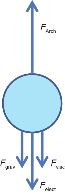
Fig. 4. Momentum contributions associated with a single water droplet.

• The Archimedes contribution: This accounts for the buoyancy of the water droplet suspended in the crude oil.

• The  viscosity  contribution:  This  opposes  the  droplet  motion(variable direction).

• The gravity contribution: This is the driving force for the separation of the water and oil phases.

• The electrostatic contribution: This favors the coalescence of the droplets (variable direction).

where V_p  is the volume of the single water droplet (in m³ ); ρ_oil  and ρ_water  are the densities of the oil and water (in kg·m^-3),  respectively;  g is gravity, with g = 9.81 m·s⁻²; C_D is the frictional factor of a droplet in laminar conditions (24/Re); v is the falling/rising velocity of  the water droplet (in m·s⁻¹); A_p is  the  droplet  section  orthogonal to the droplet direction (in m²); ε₀ is the electrical constant, with ε₀ = 8.85 × 10⁻¹² F·m⁻¹; ε_r is the water/oil electrical constant; E is the intensity of the electrical field (in V·m⁻¹ ); dist means the distance between two droplets (in m); and d p is the diameter of the droplet (in m).

Supposing that the electrical field is not present, it is possible to calculate the critical diameter that zeroes the momentum balance on the water droplet along the vertical coordinate, thus obtaining the Stokes’ law for droplets in laminar flows:

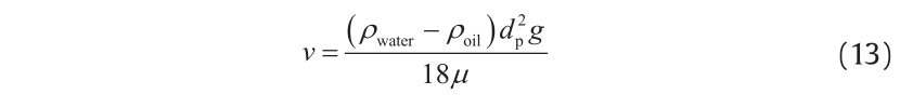
Note  that  this  equation  permits  an  evaluation  of  the  critical droplet diameter when the oil velocity equals the droplet velocity (this is roughly the definition of critical droplet diameter). The oil velocity is calculated as the ratio between the volumetric flow and the cross-sectional area of the coalescer. By zeroing Eq. (13) in the diameter of the droplet dp, the critical diameter is obtained. Assuming standard oil properties and typical convective velocity of industrial cases (2.5 mm·s⁻¹ ), the critical diameter of the water droplet is 335 µm. This value for the critical droplet diameter may be slightly overestimated because Eq. (13) assumes that the droplet is spherical.

Three different scenarios may arise:

（1）The water droplet diameter is smaller than the critical diameter. This means that the gravity contribution is not enough to win over the force induced by the oil velocity. Thus, small droplets are dragged to the top of the coalescer. The electrical field must be effective on these droplets.

（2）The water droplet diameter matches the critical diameter. The droplet is at a steady elevation in the coalescer within the oil flow. This happens when the gravity contribution equals the force induced by the oil velocity.

（3）The water droplet diameter is larger than the critical diameter. The gravity contribution is larger than the other contributions, and the water droplet moves to the bottom of the coalescer, separating the water phase from the oil. Droplets with  large  diameters  do  not  benefit  from  the  presence  of electrical  fields,  but  their  formation  from  smaller  droplets is strongly favored by electrical fields. However, too-intense electrical fields can destroy large droplets and thus generate a multitude of small droplets, significantly decreasing the coalescer efficiency. (We will describe this situation later.)

An effective coalescer has the task of favoring, first, the formation, and second, the separation, of  large water droplets. An important contribution comes from the electrical field (Eq. (12)). To characterize the presence of the electrical field, the relative distance between two droplets is required. Such information is not easily available in the literature. Therefore, a regular cubic distribution(Fig. 5) of the water droplets in the continuous oil phase is assumed.

《Fig. 5》

Fig. 5. Regular cubic distribution of water droplets.

Given the water concentration in the crude oil feedstock, it is sufficient to use the relative volumes of the phases to calculate the average distance between two droplets (where conc is the dimensionless molar ratio and d_p  is the critical droplet diameter):

The variation of the critical droplet diameter with respect to the oil convection velocity is obtained through the modified Stokes’ law:

and reported in Fig. 6. Small variations of the oil speed induce significant variations in the critical droplet diameter. An increase in the oil speed leads to a decrease of the coalescer efficiency.

《Fig. 6》

Fig. 6. Variation of the critical droplet diameter (ordinate axis) with the oil velocity.

The attraction velocity of two droplets subject to the electrical field is

and the collision time and height are, respectively:

Note that the collisions are assumed to occur along the oil direction only. Varying the voltage causes the collision height (Fig. 7) to decrease. The largest variations are obtained up to about 25 kV, and then the trend moves asymptotically to zero with higher voltages. Modern industrial applications adopt 20–30 kV. Analogously, the collision time decreases, reducing the residence time of the industrial coalescer (by 30–90 min). Collision height also varies with the inlet water concentration (Fig. 8). The collision height decreases with higher water concentrations in the feedstock. This is because of the thicker concentration of water droplets in the oil, assuming that their  diameter  is  unchanged,  with  a  consequent  reduction  of  the distance among them (inversely proportional to the cubic root of the concentration). Obviously, imposing an upper limit for water concentration ensures the safe operation of the electrostatic coalescer.

《Fig. 7》

Fig. 7. Variation of the collision height with the voltage.

《Fig. 8》

Fig. 8. Variation of the collision height with the inlet water concentration (voltage 20 kV).

《3.3. Dimensional distribution of the water droplets》

3.3. Dimensional distribution of the water droplets

Higher prevision accuracy  and  model  flexibility  are  achieved by introducing  a  dimensional  distribution  of  the  water  droplets. In practice, the assumption of regular (cubic) distributions of the droplets in the crude oil is removed, and the droplet diameter distribution is accounted for, according to the real conditions of the upstream operations. The total volume of oil can be calculated when the inlet water concentration is given:

where Vol_oil is the oil volume within the coalescer; conc(z) is the total water concentration at the coalescer height z; and ρ_oil is the oil density.

Once the oil volume around the droplets is known, it is possible to calculate the ratio between the water droplet diameter and the corresponding oil droplet with respect to the height z (Fig. 9):

《Fig. 9》

Fig. 9. Hypothesis of spatial distribution of water droplets (concentration 3% v/v).

The diameter ratio allows the calculation of the distance between the water droplets in the emulsion, and thus the characterization of the heterogeneous nature of the fluid within the coalescer. The water droplets within the water in an oil emulsion can have a wide range of diameters, from 0.1 µm to several millimeters. It is reasonable to discretize the distribution into several classes of diameters. For example, a population of water droplets with diameters from 75 µm to 300 µm can be split into N classes of 25 µm:

Each class will be initially populated according to the inlet distribution of diameters, which may be estimated according to heuristic methodologies or computed in a random fashion. In the latter case, the random distribution of diameters ensures mass conservation at the inlet section of the coalescer. Given the initial distribution of diameters, the system dynamics will lead to a decrease in the amount of water droplets within the coalescer and a gradual increase in the classes with higher diameters due to the coalescence (Fig. 10).

《Fig. 10》

Fig. 10. Population of water droplets and classes of diameters, with the last class including the critical diameter.

It is worth emphasizing that the last class, N, must have the critical droplet diameter as the right extreme of the interval.

《3.4. Coalescence》

3.4. Coalescence

The discretization of the droplet distribution allows a simplified modeling of the coalescence phenomenon. When considering a single droplet, coalescence leads to an increase in the droplet dimensions until the critical diameter is achieved and overcome. Gravity and electrostatic contributions favor the coalescence. Each class of diameters  has  a  specific  “coefficient  of  coalescence”  with  respect   to all the other classes. This coefficient, f (i, j), of the class i with respect to the class j, accounts for the effectiveness of the impacts between two droplets in terms of coalescence. The evaluation of f (i, j) is addressed with the equations listed below (Eqs. (22–24)). Note that these equations require an adaptive coefficient (φ), which is estimated experimentally. In this study, the value of φ equals 0.001. Nevertheless, this parameter can assume different values according to the use of chemicals and additives to favor coalescence.

To clarify this concept, consider the effective coalescence due to the collision of two droplets belonging to the classes i and j, respectively. Their collision is proportional to the relative velocity and the distance:

where FDI is the frequency of collisions between two water droplets; v is the droplet velocity of classes i and j; and D_nom is the nomi-nal diameter of the classes i and j.

FDI also requires an efficiency of collisions that can be related to the difference of the nominal diameters of the droplet classes:

Apart from the adaptive parameter φ, the coalescence factor can be stated as follows:

where Φ(E) is the electrostatic contribution. The  resulting  coalescence  triangular  matrix  that  contains  all  the  coalescence  factors must be recalculated at each integration step, continuously updating the water concentration within the coalescer.

《3.5. Mathematical model》

3.5. Mathematical model

The previous formulations must be adopted to simulate the performance of electrostatic coalescer units; finally, appropriate balances for the mass and number of droplets based on the conservation principle must be defined to characterize the evolution of the system.

The falling velocity of large droplets is due to the contribution of gravity. In viscous flow, this results in a falling velocity of

where Δρ is the difference between the densities of the water and oil (in kg·m⁻³); d is the diameter of the ith droplet (in m); and μ is the dynamic viscosity of water (in cP).

The droplet velocity due to the electrical field is derived from the attraction force:

where ε₀ is the void electrical permittivity (in F·m⁻¹ ); ε_water is the water electrical permittivity (in F·m⁻¹ ); ε_oil is the oil electrical permittivity (in F·m ¹ ); E is the electrical field (in V·m⁻¹ ); d _i and d _j are the diameters of the ith and jth droplets (in m), respectively; and dist _i,j is the distance between the two droplets (in m).

As a result, two droplets are accelerated because of their attraction:

where d_av is the average diameter. Therefore, the velocity that accounts for the gravity and electrostatic contributions of the droplet i, which is attracted to droplet j with a resistance generated by the oil velocity, is stated as follows:

Suppose that the electrical field is in the direction of the oil flow. Moreover, suppose that a droplet with diameter d_i is attracted by a droplet of the same class immediately beneath it at a distance dist:

The following limit velocity is obtained:

Assuming that the volumetric fraction of the water is X, the average distance between droplets is

Substituting this value into Eq. (30) results in the following:

By imposing v _lim = 0, a quadratic function is obtained; its positive solution is the diameter that zeroes the rising velocity. Such a diameter is called the critical diameter (d_cri ); d_cri is univocally defined in the water-oil system as a function of the electrical field, the concentration of water, and the oil velocity. The coalescence coefficients are calculated as follows (this is a simplified version of Eq. (24)):

which has the same dimensions as those of a frequency (i.e., 1 s⁻¹ ). The variables v _i and v _j represent the limit velocities, dist _i,j is the distance, and φ _i,j is the collision effectiveness. The relative difference of the velocities of droplets i and j is given by the sum of the gravity and electrostatic contributions.

With these modifications, it is possible to define the mass and droplet number balances for the classes to complete the mathematical model. All the droplets move from the bottom to the top of the coalescer, except for the droplets of the class N, which are characterized by the critical diameter. These move from the top to the bottom of the coalescer. As a result, the droplets with critical diameter thatoriginate at a certain height in the coalescer will invert their direction and start falling, whereas the remaining droplets will proceed toward the top of the unit. It is possible to foresee that the resulting numerical problem is a boundary value problem that can be solved with iterative procedures.

The balance for the ith class of droplets involves different terms. The number of droplets can decrease for the collisions caused by droplets i with droplets of higher (or the same) classes. The number of droplets can also decrease for the collisions caused by smaller

droplets coming from lower classes. In summary, the decrease of droplets of the ith class is stated as follows:

The collision of droplets i and j generates a droplet with a larger diameter, obtained from the conservation principle.

The number of droplets of the ith class can increase only if two droplets of lower classes collide, generating a new droplet with diameter d_i. The generation is described as follows:

and it is valid only for the couple of droplets that, colliding, produce droplets with diameter d _i .

Thus, the ith droplet variation can be expressed as follows:

and the variation in the mass of the corresponding class of droplets is given by

where kC _i is the overall mass of the ith class and kg _i is the mass of the single droplet.

Assuming that the reference system for the time coordinate is consistent with the oil flow, which has velocity v_oil :

《4.Robust numerical solution》

4.Robust numerical solution

Given:

• The grid distance, which is assumed to be the total height of the unit;

• The oil flow rate;

• The water collector surface, which is assumed to be the crosssectional area of the coalescer;

• The volumetric concentration of water droplets;

• The diameter distribution of water droplets;

• The temperature, which the oil density and viscosity  depend on; and

• The intensity of the electrical field.

It is possible  to evaluate all  the terms within  the differential equations of the balances (Eqs. (37) and (38)). The system can be easily integrated using explicit methods (Euler and the fourth-order Runge-Kutta, for comparison). The use of implicit methods is surely possible, and is a valid alternative [17].

The resulting problem consists of about 50 classes and about 1000 integration steps, leading to a system with 50 000 equations and sparse Jacobian and tridiagonal blocks structure, where blocks are 50 × 50. The integration step is derived from the following:

assuming that dz = 1 mm is reasonable, if it is considered to correspond to the average distance of two droplets with a diameter of 300 µm and with 3% of the initial concentration of water in oil. The integration is carried out from t = 0 to the overall residence time:

As mentioned above, the problem is with boundary conditions, and is brought back to the iterative solution and convergence to initial conditions. In practice, only the distribution of the inlet mass flows is known, whereas the water flow of the class N coming from the different layers of the coalescer is unknown. It is necessary to estimate the profile of the flows of the class N and update it at each iteration. The procedure is as follows:

Step 1: Define with KN _j the total flow of the class N outflowing the layer j, where j = 1, …, P and P is the number of integration steps. Note that KN _j represents the sum of the flow that enters the jth layer plus the quantity produced locally.

Step 2: Make the initial assumption that KN _j = 0 for all the layers. For the sake of simplicity, KNa _j indicates the assigned values.

Step 3: Solve the differential system, evaluating the profile KNc_j of the calculated values.

Step 4: If all KNc_j are null, the calculation is stopped, since the separation efficiency is null (no droplets achieve the critical diameter).

Step 5: Otherwise, assume

and proceed with a new integration loop. The calculations end when the overall balances are satisfied.

The proposed numerical procedure is stable, although the computational effort is not negligible. It is possible to speed up the computations by adopting the following device. It is possible to indicate with

the separated water evaluated as the difference between the inlet water (inlet) and the remaining water obtained at the end of the integration loop (drag). As it is defined, KNc₁ represents the same quantity calculated at the end of the integration loop. Thus, by imposing

it is possible to redefine

for all the layers j = 1, …, P; the convergence is then quickly achieved with 5–6 iterations and 0.1% of error on the balance consistency,

《5.Results and sensitivity analysis》

5.Results and sensitivity analysis

According to the mathematical modeling proposed in the previous sections, the sensitivity analysis of the electrostatic coalescer is performed with respect to the main parameters: inlet flow rate, inlet water concentration, voltage, height of the coalescer, and diameter distribution of water droplets.

Typical operating conditions are selected for the sensitivity analysis (Table 1). The diameter distribution of the water droplets is selected according to the literature and experimental evidence [18]: 95% of the droplets have diameters of 50 µm, and the remaining 5% of 100 µm.

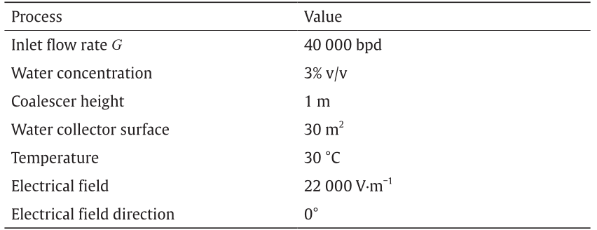
《Table 1》

Table 1 Operational parameters.

The model evaluates the critical diameter (223.26 µm), the inlet water flow (495 kg), the water separated from oil (272.6 kg), the remaining water in oil (222.4 kg), the outlet water concentration (1.347%), the coalescer efficiency (55.1%), and the residence time (224 s). Fig. 11 illustrates the dynamics of the classes of droplet diameters. The smallest droplets progressively disappear, despite larger and larger diameters occurring with respect to the coalescer height (residence time), until the largest diameter considered (which is necessarily larger than the critical diameter) is achieved. It is worth noting that the class with the smallest diameter has a typical firstorder response, from the highest value to a horizontal asymptote. Conversely, the intermediate classes selected present an overshot; in fact, they can be considered as intermediate products between the starting classes, which are characterized by smaller diameters, and the last class, which has the largest diameter, to which all other classes are tending. The behavior of the last class corroborates the considerations above since it monotonically increases according to highorder dynamics response. The simulation of Fig. 11 will be considered as the base case for the following sensitivity analysis.

《Fig. 11》

Fig. 11. Some key classes of droplet diameters, with respect to the coalescer height.

《5.1. Voltage》

5.1. Voltage

The intensity of the electrical field can significantly modify the behavior and performance of the entire coalescer. The selected distribution has an upper bound of 27 kV; beyond this limit, voltage destroys the droplets, thus generating a large number of droplets with very small diameters that cannot coalesce in any way within the unit. Analogously, a lower bound is also defined, since the coalescer performances are poor when the electrical field is lower than 18 kV. Fig. 12 reports the coalescer efficiency within the operational range of the voltage. It varies from 61.1% at 18 kV to 80.4% at 26 kV. The increase is almost linear and the overall efficiency cannot be further improved by increasing the voltage due to the need to preserve the integrity of the water droplets. Fig. 13 shows the decrease of the water concentration in the oil outflowing the coalescer with respect to the increase of the voltage. The concentration is almost halved from 18 kV to 26 kV. With the same quantity of water in the feed flow rate, the higher the voltage, the better the coalescer performs, within the operational range. The temporal evolution of the system is also influenced by the voltage. The coalescence of the water droplets is quite small without the voltage (Fig. 14): The volume of the smallest droplets slightly decreases (a variation smaller than 10%), whereas the classes of larger diameters show negligible variations (1%–2%). The dynamics with the lowest voltage allowed, 18 kV, as reported in Fig. 15, are more interesting. The water droplets with diameters of 195‒200 µm overcome the 5% v/v, whereas the volume of the 45‒50 µm droplets drops to less than 0.5% v/v. With the highest voltage, as shown in Fig. 16, the coalescence is the main phenomenon. Note that the last class of droplet diameters is no longer 195‒200 µm, since it is larger than the critical diameter related to these operating conditions; the top class is 170 µm. The smallest droplets immediately coalesce, and their trend is also excluded from the picture.

《Fig. 12》

Fig. 12. Coalescer efficiency (outlet water/inlet water) with respect to the voltage.

《Fig. 13》

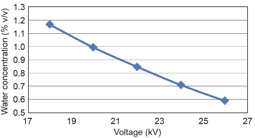
Fig. 13. Water concentration in oil exiting the coalescer with respect to the voltage.

《Fig. 14》

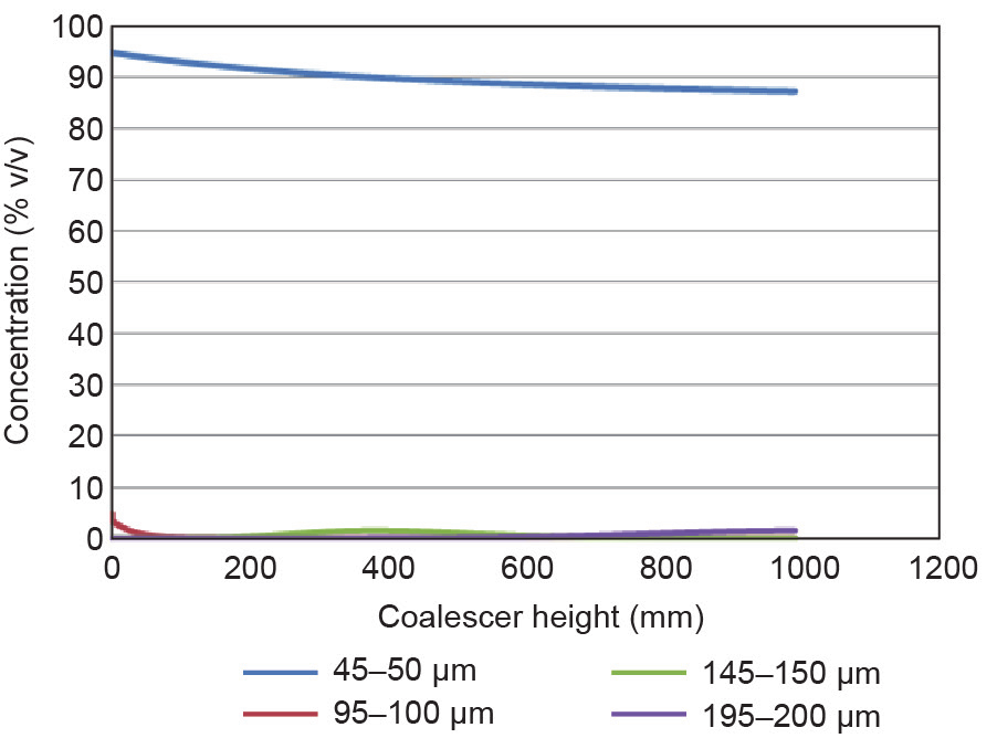
Fig. 14. Classes of droplet diameters with respect to the coalescer height without voltage  (0  kV).

《Fig. 15》

Fig. 15. Classes of droplet diameters with respect to the coalescer height with the lowest voltage (18 kV).

《Fig. 16》

Fig. 16. Classes of droplet diameters with respect to the coalescer height with the highest voltage (26 kV).

《5.2. Concentration》

5.2. Concentration

The concentration of water in the feedstock is another parameter that can strongly modify the behavior and efficiency of the electrostatic coalescer. Fig. 17 shows that the efficiency of the overall coalescer is dramatically sensitive to the inlet water concentration. A variation from 1% v/v to 2% v/v in the inlet water concentration leads to an efficiency increase of about 40%. This is because emulsions with smaller concentrations of water unavoidably lead to larger distances between the water droplets and, therefore, to less-effective coalescence. Fig. 18 shows that the outlet concentration of water in oil has a maximum that is relatively close to the 2% v/v inlet water concentration. In fact, with intermediate concentrations of water in the inlet flow rate, the droplet-falling effect is rather small. Therefore, an increase in the concentration of the water in the feedstock corresponds to an increase in the outlet water still contained in the oil. After a water concentration limit of about 2%, the droplet-falling effect becomes dominant and an increase in the inlet water concentration leads to a decrease in the outlet water concentration in oil. The best industrial practice exploits this behavior by supplying additional water when the worst condition of 2% inlet water concentration occurs. Moreover, the additional water could be supplied as large droplets from the top of the unit, to favor the falling effect and improve the coalescer efficiency. Analogously to the previous analysis, the dynamics of the classes of droplet diameters significantly changes (Fig. 19). With reduced water inlet concentrations (1%–2% v/v), the coalescence of the smallest droplets is relatively slow and the volume of the larger droplets remains particularly small along the unit height. When the inlet water concentration is larger (3%–4% v/v), the coalescence of small droplets is faster and larger, and larger droplets are generated, favoring the phase separation. This result can be clearly seen when looking at the overshot of the intermediate classes in Fig. 19. The droplets with diameters of 145‒150 µm achieve their maximum volume of 6% at the relative height of 250 mm, with 1% v/v inlet water concentration. With 2% v/v inlet water concentration, the maximum volume is achieved at 150 mm of the coalescer height. Moreover, the decreasing trend after this maximum is much faster than the previous one at 1% v/v inlet water concentration. With 3% v/v inlet water concentration, the maximum volume is achieved at 50 mm of the coalescer height. Unfortunately, the volume decreases more slowly than in the previous cases, despite classes with larger diameters. This result is because the critical diameter is gradually decreasing with the increase of inlet water concentration, and this class is approaching the limit. In fact, with 4% v/v inlet water concentration, the class with the largest droplets has a diameter of 170 µm.

《Fig. 17》

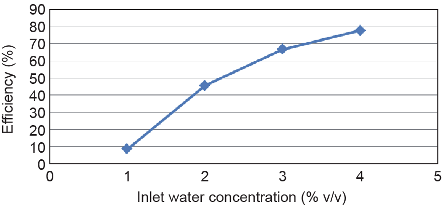
Fig. 17. Coalescer efficiency with respect to the inlet water concentration.

《Fig. 18》

Fig. 18. Outlet concentration of water in oil with respect to the inlet water concentration.

《Fig. 19》

Fig. 19. Classes of droplet diameters with respect to the coalescer height in different inlet water concentrations. (a) 1% v/v; (b) 2% v/v; (c) 3% v/v; (d) 4% v/v.

《5.3. Grid distance (coalescer height)》

5.3. Grid distance (coalescer height)

The electrical grid distance is usually considered to be the active height of the electrostatic coalescer. It defines the geometry of the coalescer and the residence time of the emulsion. The grids must be placed at an adequate distance that is a good compromise between good efficiencies (Fig. 20) and reasonable unit design. Small distances (less than 400–500 mm) could be ineffective, whereas large distances lead to unrealistic volumes for the coalescer. The water content of the outflowing oil are inversely proportional to the grid distance (Fig. 21). As expected, the trend of the classes of droplet diameters does not suffer from the variations in the grid distance, since the trends are simply stopped at different heights, with consequent different efficiencies.

《Fig. 20》

Fig. 20. Coalescer efficiency with respect to the grid distance (coalescer height).

《Fig. 21》

Fig. 21. Outlet concentration of water in oil with respect to the grid distance (coalescer height).

《5.4. Diameter distribution》

5.4. Diameter distribution

The diameter distribution adopted in the base simulation is close to the real conditions. Nevertheless, some differences in the expected value and the variance of the droplet are expected when varying the operational conditions, the geometry of the unit operation, and the properties of the feedstock. To assess the sensitivity of the system, the following distribution is selected:

•  50 µm: 0%

•  100 µm: 0%

•  150 µm: 50%

•  200 µm: 20%

•  250 µm: 30%

which is strongly (and intentionally) unbalanced toward large diameters. The numerical results of the simulation are: the critical diameter (223.26 µm), inlet water flow (900 kg), water separated from oil (862.7 kg), remaining water in oil (37.3 kg), outlet water concentration (0.123%), coalescer efficiency (95.9%), and residence time (408 s). As expected, the water removal is very efficient, thanks to the ideal initial condition of large diameters of the droplets of water.

《6.Conclusions》

6.Conclusions

This research activity has addressed the first-principle mathematical modeling of electrostatic coalescer units. The model was developed  starting  from  the  fundamental  laws,  and  accounts  for the main phenomena that govern the separation of water-in-oil emulsions. Dependencies of the coalescer separation performance with respect to the voltage, the inlet water concentration, the grid distance, and the water droplet diameter distribution have been assessed and quantified. Moreover, the critical diameter of water droplets and the electrical field threshold to prevent droplet breaking have been included in the model, together with their dependencies with the operating conditions and the other relevant parameters. As a result, this mathematical model is rather flexible in its description of coalescer units in a wide range of operative variables, and can be adopted for design and operational purposes.

《Acknowledgements》

Acknowledgements

The authors gratefully thank Ing. Matteo Bruni for his activities during the M.Sc. thesis project, as well as DG Impianti Industriali SpA for the industrial support.

《Compliance with ethics guidelines》

Compliance with ethics guidelines

Francesco Rossi, Simone Colombo, Sauro Pierucci, Eliseo Ranzi, and Flavio Manenti declare that they have no conflict of interest or financial conflicts to disclose.