《1.Introduction》

1.Introduction

Carbon dioxide (CO₂) is the dominant greenhouse gas emitted by power plants. Amine-based post-combustion carbon capture is a promising technology for large-scale carbon capture, since it permits carbon capture to be achieved with a relatively simple retrofit of a conventional fossil-fuel power plant [1]. Monoethanolamine (MEA), classified as a primary amine, is the most applicable solvent when adopting a solvent-based carbon-capture strategy because it has a fast reaction rate with CO₂  as compared with secondary and tertiary amines [2]. Previous studies focused on the optimal operation of the solvent-based carbon-capture process under a specified capture level [1,3‒7]. Nonetheless, regeneration of MEA for carbon capture is energy-intensive and costly. Operation of the carbon-capture process with a constant capture level is uneconomical under the CO₂ allowance market, where the settlement price may change for every quarter auction. In Refs. [8,9], it was already noted that the CO₂ capture level might change under different CO₂ price conditions. Those CO₂ pricing mechanisms, however, are similar to a carbon tax [10]. For  a  flexible  market-oriented  CO₂   allowance  trading  mechanism [11–13], the decision maker should decide on the CO₂   allowances bid from the market. It is imperative to design a unified bidding and operation strategy for a power plant with carbon capture in order to maximize profits during the life cycle of the plant.

In this paper, we implement the Sarsa temporal-difference (TD) algorithm to explore a bidding and operation strategy for the decision maker of a specific power plant with solvent-based carbon capture. The relationship between bidding and operation is established with a holding account of the decision maker under the time-varying allowance market [14]. The performance of the strategy is assessed in terms of the discounted cumulative profit — that is, the discounted cash flow of the power plant [9]. The paper is organized as follows. In Section 2, the bidding and operation problem of a coal-fired power plant integrated with solvent-based carbon capture is discussed and formulated, based on a profit model of a coal-fired power plant integrated with a carbon-capture process that considers the quarter-based CO₂ allowance auctions. In Section 3, the Sarsa TD algorithm is introduced and applied to find an optimal solution for the aforementioned integrated system. In Section 4, the results demonstrate that the Sarsa TD algorithm can find a solution for the unified bidding and operation strategy that maximizes the profits for the specific power plant. Conclusions are drawn at the end of the paper.

《2.Problem formulation》

2.Problem formulation

In this section, a profit model of a coal-fired power plant integrated with a carbon-capture process is developed and a simplified greenhouse gas emission trading system is introduced. An objective function is then formulated in terms of the discounted cumulative profit of the power plant within the lifetime of the plant under the emission trading system.

《2.1. Development of an MEA-based carbon-capture model》

2.1. Development of an MEA-based carbon-capture model

The process model for the MEA-based carbon-capture process was developed in Aspen Plus^®[15]. Its physical properties were calculat ed using the electrolyte  non-random two-liquid (eNRTL)  method. It was validated using experimental data from pilot plants [16], and was scaled up to deal with flue gas equivalent to that discharged by a 650 MW coal-fired subcritical power plant. Fig. 1 [6,17] displays the MEA-based post-combustion carbon-capture process flow diagram. As shown in the diagram, two absorber columns are constructed for the flue gas CO₂ absorption [18]; Table 1 shows the parameters of absorber and stripper columns. A lean MEA solvent stream is divided into two equal parts by Splitter 1 and fed into the top of  two absorbers. Simultaneously, the flue gas from a power plant is divided by Splitter 2 and injected into the bottom of the absorbers. In the absorber columns, CO₂ in the flue gas reacts with the MEA solvent automatically. The vapor phase, which has less CO₂, is released into the atmosphere, while the MEA solvent phase, which is rich in CO₂, is pumped to the cross heat exchanger and then transported to the stripper. In the stripper column, CO₂  is decomposed from the rich MEA solvent, while a lean MEA solvent is regenerated and leaves the stripper bottom. This lean MEA solvent is cooled by the cross heat exchanger and the downstream cooler, since it should achieve a specified temperature target of the inlet lean MEA solvent of the two absorbers. In addition, before recycling, MEA and water losses are made up using Mixer 3. Eventually, the lean MEA solvent is fed back for continuous CO₂ absorption. Through the condenser of the stripper, a high-concentration CO₂ product is ready for compression and transport.

In Fig. 1, the MEA-based post-combustion carbon-capture process is controlled by four control loops. A similar control scheme is discussed in the literature [3,17]. Correspondingly, for the steady-state model in Aspen Plus^®, we set the design specifications as follows: ① The top stage temperature of the stripper is set at 35 °C by varying the condenser duty; ② the temperature of the lean MEA solvent at the top of the absorbers is set at 40 °C by varying the cooler duty; ③ the lean loading (i.e., the mole ratio between CO₂ and MEA in lean MEA solvent) of lean MEA solvent is set at around 0.2 mol of CO₂ per mol of MEA ( ) [18,19] by varying the reboiler heat duty; and ④ the CO₂ capture level should be set at a specified value within a discrete value set {50%, 60%, 70%, 80%, 90%} by manipulating the lean MEA flow rate. Note that, in reality, since lean loading is difficult to measure, the reboiler temperature is specified by varying the heat duty that indicates lean loading.

《Fig. 1》

Fig. 1. The MEA-based post-combustion carbon-capture process flow diagram [6,17]. AT: composition transmitter; FT: flow transmitter; TT: temperature transmitter; CC: CO₂ capture  level  controller;  LLC:  lean  loading  controller;  TC:  temperature  controller.

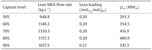
With the  specifications  of  the absorber  and  stripper  columns as shown in Table 1 and the base input settings of the flue gas and lean MEA solvent as shown in Table 2, we further manipulate the mole flowrate and lean loading of the lean MEA solvent to achieve specified  CO₂ capture levels with the least reboiler duties. Table 3 summarizes the performance for each operation specification, from which we can determine the optimal reboiler duty Q_reb  (c_t) for different CO₂ capture levels c_t in the tth quarter.

《Table 1》

Table 1 Parameters of absorber and stripper columns.

《Table 2》

Table 2 Material streams of post-combustion carbon capture.

《Table 3》

Table 3 Performance of the MEA-based post-combustion carbon-capture process with different operation specifications.

《2.2. Profit model for coal-fired subcritical power plant》

2.2. Profit model for coal-fired subcritical power plant

Coal-fired power plants are important elements since they contribute to major energy consumption around the world and release the most CO₂   of any power generation systems [20]. Therefore, in this section, we formulate the quarterly profit for a coal-fired subcritical power plant that is integrated with carbon capture. We also establish the relationship between the operation specifications and the electricity output. According to the US Energy Information Administration (EIA) [21], the cost, C_t, of a power plant for the tth quarter in USD per quarter (USD·qtr^–1) can be calculated as follows:

where FOM is the quarterly fixed operation and maintenance (OM) cost; VOM_t  is the quarterly variable OM cost; F_t  is the quarterly fuel cost; and B_t  is the quarterly CO₂ bidding cost. According to the Cal ifornia CO₂ allowance auction mechanism [11], the bidding cost is defined as follows:

where v_t is the settlement price of CO₂ allowances in USD per allowance for a quarterly allowance auction and w_t is the winning CO₂ allowances of the decision maker for the tth quarter. One CO₂ allowance permits the release of one metric ton of CO₂  by a power plant. Other items in Eq. (1) are summarized below:

where β and δ are fixed and variable OM cost coefficients, respectively; f is the fuel cost; and P_n is the power plant nominal capacity. These variables are defined in Table 4 [21] with specific units. In addition, Et  is the electricity output (kW·h·qtr^-1 )and H_t  is the fuel consumption (GJ·qtr^–1). The revenue from the electricity generation of a coal-fired power plant can be written as follows：

《Table 4》

Table 4 Parameters of a power plant with carbon capture [21].

where λ is the electricity price in USD·(kW·h)^–1, shown in Table 4. The profit for the tth quarter can be then derived as follows:

where we denote P_t = P (E_t, H_t, w_t, v_t) since the profit is dependent on the variables E_t, H_t, w_t, and v_t .

In this paper, the total fuel consumption for power generation and carbon capture, H_t, is assumed to be constant. As a result, tradeoffs should be made between the electricity output of the main power plant and the energy-intensive carbon capture for the integrated carbon-capture facilities. For a coal-fired power plant with nominal capacity P_n  = 650 000 kW, as specified in Table 4, the fuel nominal capacity Pn  = 650 000 kW, as specified in Table 4, the fuel consumption in a quarter can be calculated as follows:

where the value 2190 represents the number of hours in one quarter. The quarterly energy consumption of the carbon capture, U_t, in GJ·qtr^–1, is constrained by

U_t  can be related to the corresponding reboiler duty, Q_reb(c_t), as discussed in Section 2.1:

By combining Eqs. (9) and (10), the electricity output E_t  for the tth quarter can be derived as follows:

which indicates that the capture level ct can uniquely determine the electricity output. The quarterly profit of the power plant (Eq. (7)) can be simplified as follows:

In summary, for a specific coal-fired power plant with CO₂   capture, assuming a fixed amount of fuel to be used and continually fixed fuel and electricity prices, its profit Pt  for the tth quarter can be uniquely determined by the CO₂ capture level c_t, the winning CO₂ allowances of the decision maker w_t purchased from the CO₂ auction, and the settlement price v_t  for each CO₂  allowance.

《2.3.CO2 allowance market》

2.3.CO₂ allowance market

In Section 2.2, although the profit, P_t (Eq. (7)), for one quarter is fully defined, only two degrees of freedom, E_t and H_t, have been discussed. The other two degrees of freedom, wt and vt, should be influenced by the CO₂ allowance market conditions. A quarterly market condition will be fully defined when the bid options (including bid quantities q and bid prices p) of all covered or opt-in entities (e.g., power generation companies) in the market are submitted to the auction operator. The bid quantity and bid price of the entity concerning the decision maker are denoted as q_0,t and p_0,t, respectively; the bid quantities and prices for all the other entities are denoted as q_i,t and p_i,t, respectively, for i ∈ I, where I={1, 2, 3, …, I} is the entity set of all the covered entities in the allowance market except the entity of the decision maker. The operator will then implement the sealed bid auction mechanism [14] as follows.

During one quarter, the auction operator will reject unqualified bids that violate the purchase limit, holding limit, or bid guarantee of the corresponding entity or bidder. Subsequently, the qualified bids of all bidders will be considered by descending order in terms of  bid prices.  Beginning  with the  highest  price bid,  bidders submitting bids at each price will be sold CO₂  allowances equivalent to their bid quantities until one of the following conditions applies: All the auctioned allowances, A, in the allowance market are sold out; or, the bid price of the next bidder is less than the auction reserve price, gt, in USD per allowance [11]. If the auctioned CO₂ allowances are sold out, the settlement price is the bid price for the last bid that is sold with allowances; if the settlement price is equal to the reserve price, the sold CO₂ allowances are the cumulative bid quantities of all the bids with prices above the price of the reserve bid. The auction operator can then calculate the winning CO₂ allowances of the winning bid of each bidder or entity (e.g., the winning CO₂ allowance of the decision maker is w_t in this paper), the sold CO₂ allowances u_t, and the unified settlement price v_t for all entities, where

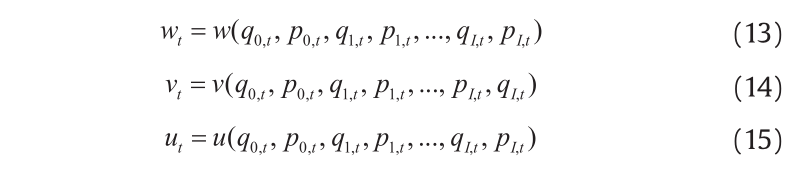
In Eqs. (13), (14), or (15), the decision maker can only determine its own bid quantity q_0,t  and bid price p_0,t. The decision maker should   estimate the bid options for other companies using the historical bidding data of other entities, as represented by the probabilities shown in Section 2.4.

In this paper, in order to judge whether a bid is qualified or not, we only consider the holding limit, h_l, of the power plant decision maker in the allowances. The purchase limit and bid guarantee are omitted for simplicity. The holding limit is the upper limit of a holding account for an entity that is covered in the allowance markets. If the submitted bid quantity, q, of any entity may latently cause its holding  account  CO₂   allowances  to  exceed  the  holding  limit,  this submitted bid will be an unqualified bid and will be rejected by the auction operator. In this paper, the holding account only has an analogous functionality of several accounts, as set forth in the California code of regulations [11]. We assume the following constraints for holding account CO₂  allowances:

where h_t+1 is the holding account CO₂  allowances at the beginning of the (t+1)th quarter auction. Note that if winning CO₂ allowances, w_t, are less than the CO₂ emission, e_t, extra CO₂ allowances should be surrendered from  the holding account;  if the  winning CO₂ allowances are more than the CO₂  emission, the redundant winning CO₂ allowances will be reserved in the holding account. The total CO₂ allowances accumulated in the holding account for all quarters before the tth quarter is denoted as h_t. The inequality in Eq. (17) indicates that the holding account CO₂  allowances, h_t, should not be exhausted; otherwise, extra penalties will be paid due to excess emissions without the surrender of allowances. According to the California regulations [11], four times the excess emission is set as the compliance obligation for untimely surrender. Additional bidding and trading mechanisms will be introduced to meet the untimely surrender obligation. For brevity, we assume that the penalty of untimely surrender is 320 USD for each metric ton of CO₂ excess emission, rather than the penalty set forth in the California regulations. Therefore, the inequality in Eq. (17) is a soft bound. On the other hand, the inequality in Eq. (16) implies that, for any t, the decision maker should only submit bid quantity q_0,t, which may not potentially cause h_t+1 greater than h_l, as mentioned earlier. The variable e_t  represents the CO₂  emission of the power plant in the tth quarter in t·qtr^-1 which can be determined as follows:

Since c_t  is the CO₂   capture level related to the operation of the solvent-based carbon-capture process, while w_t and q_0,t  are related to the bidding under the CO₂  allowance market, the inequalities in Eqs. (16) and (17) indicate the latent relationship between bidding and operation.

《2.4. Objective formulation》

2.4. Objective formulation

In Section 2.2, the profit (Eq. (12)) is expressed by the CO₂  capture level c_t, the winning CO₂ allowances of the decision maker w_t, and the settlement price v_t. The capture level, c_t, can be arbitrarily determined by the decision maker, while the winning CO₂ allowances, w_t, and the settlement price, v_t, must be determined by bid options of all the entities shown in Eqs. (13) and (14). Provided that all the other entities have submitted their bid options (i.e., p_i,t and q_i,t with "i ∈ I), the decision maker of the power plant with carbon capture only needs to determine the operation method, that is, c_t, and the bidding method, (q_0,t, p_0,t), for the corresponding profit (Eq. (12)) estimation. The unified action is denoted as

where A(s_t) is the discrete action set under state s_t and is supposed to be A for. Note that the decision maker for the power plant only knows its own bidding quantity, q_0,t, and price, p_0,t; q_i,t and p_i,t of other bidders for i ∈ I must be estimated by the decision maker using a priori knowledge. In this paper, the bid quantities and prices of other entities are presumed to be influenced by the settlement price, v_t–1, and sold allowance, u_t–1, of the last-quarter CO₂ allowance auction. A similar state-choosing method is discussed for the electricity market[22]. Thus, a state s_t in the tth quarter is denoted as follows:

where h_t is considered as a state variable in Eq. (20), since holding account CO₂ allowances should be sufficient (Eq. (17)) but not potentially exceed the holding limit h_l (Eq. (16)). Besides, we tend to maximize the discounted cumulative profit of the power plant in question within its lifetime; therefore, time t is set as a state entry so that the decision maker can take different actions in different periods of the power plant life cycle.

Supposing that the bidding quantity set and bid price set for each entity are and , respectively, the decision maker can then estimate the probability κ of any bidder choosing a possible bidding option, which is

for any i ∈ I. Note that, although an entity may choose its bid option differently in each quarter, the bid option sets for quantity and price (i.e.,  and ) are time-invariant and are assumed to be unchanged for "s. Subsequently, we construct the following Markov decision process. Under a specific state, s_t  = s, the decision maker takes a possible action a_t = a. With the joint probability defined as

all the other bidders will choose their own bidding options as specified in Eq. (22), so that the next-quarter state s_t+1 = (v_t, u_t, h_t+1, t+1) = s′ can be uniquely determined when taking action at  = a. Furthermore, a reward, r_t+1, is derived in terms of the state transition from st to s_t+1, based on Eq. (12)—that is, that

Note that “reward” is the terminology defined under the framework of the reinforcement learning (RL). Physically, the (t+1)th quarter reward, r_t+1, is the power plant profit P_t  (Eq. (12)) for the tth quarter. Since t is any time index, the decision maker can recursively obtain the finite-time horizon reward sequence as s_t, a_t, s_t+1, r_t+1, a_t+1, s_t+2, r_t+2, …, a_t+N–1, s_t+N, r_t+N, namely, an episode of bidding and operation. The variable N represents the lifetime of the power plant with the MEA-based carbon-capture process. For "k ∈ {0, 1, …, N–1}, the objective function can be constructed as

Subject to

where V ^π(s_t ) is the state-value function for state s under policy π; r_t+k+1 is the reward when transiting from state s_t+k to s_t+k+1; γ is the discount coefficient; and E_π{·} is the expectation of a discounted reward sequence under the policy π. For the decision maker, the probability of a stochastic policy is written as π (s_t+k, a_t+k), where the probability of each action, a_t+k, should be determined under each state, s_t+k, in order to maximize the lifetime discounted cumulative profit. We consider a stochastic or soft policy, since the optimal policy should be explored by the RL-based Sarsa TD algorithm. In the end, the soft policy should be gradually changed into an applicable deterministic optimal policy. Eqs. (26) and (27) can be obtained from Eqs. (16) and (17), respectively.

《3.The Sarsa TD algorithm: Introduction and implementation》

3.The Sarsa TD algorithm: Introduction and implementation

The RL-based Sarsa TD algorithm is one applicable algorithm that can find the optimal policy or strategy of the problem defined in Section 2. Such an algorithm can be programed in Matlab®. We apply this method for the power plant profit maximization, since it has adaptive and model-free features. As a result, an initial optimal policy can be found automatically with respect to a modeled environment in Section 2; further policy adjustment can be made when the agent for the decision-making of the power plant interacts with the real environment. The Sarsa TD algorithm requires less computation time than dynamic programming and has better convergence property than another basic RL algorithm called Q-learning [23]. Nevertheless, it should be noted that the Sarsa TD algorithm often finds a worse policy if the tuning parameters, such as ε, are scheduled improperly. The parameter ε is the probability of exploring the action set A, which will be introduced later.

To design a Sarsa TD algorithm, we should define an optimal action-value function based on Eq. (24), which is

for all s ∈ S and a ∈ A, where Q ^π is denoted as the action-value function in terms of policy π. Therefore, the optimal policy is

The optimal action value Q*, nevertheless, is unknown if the optimal policy has not yet been obtained. According to Refs. [23,24], an action value function iteration method (Eq. (30)) can ensure that the action value function Q_t+k+1 (s, a) converges to Q^π(s, a) for infinite times of visits to all states s ∈ S and all actions a ∈ A with k → ∞. The iteration method is

where a should be an action derived from the current policy π; α is the learning rate. Supposing that an estimator of Q ^π(s, a) based on Eq. (30) is , policy improvement is achieved through the following  equations:

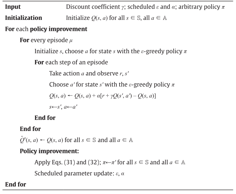
where is the greedy action causing an improved policy π' ( s, a) compared with π(s, a); n_A  is the number of possible actions in action set A; and ε is the probability of choosing any action in the action set A uniformly. All the actions except for the greedy one are called exploratory actions. The exploratory actions can ensure the finding of the optimal policy that causes global maximum state values, V^π  (Eq. (24)), in each state, rather than some local maximums. By setting the new policy as π←π′, Eqs. (30), (31), and (32) form the action value iteration algorithm that should be repeated forever. This algorithm can obtain the optimal policy, π*. Before using this algorithm, both α and ε should be scheduled. The learning rate, α, should be large to ensure fast initialization of Q(s, a) (Eq. (30)) for all s ∈ S and all a ∈A, but eventually small to make those action values convergent. Although theoretical conditions exist for the scheduled α sequence, they are seldom used in applications [23]. The probability, ε, of exploring the action set is equal to one for a fully exploratory start, but gradually decreases to zero for the final derivation of a deterministic policy. Table 5 presents the Sarsa TD algorithm with the ε-greedy policy.

《Table 5》

Table 5 The RL-based Sarsa TD algorithm with the ε-greedy policy.

Note that the Sarsa TD algorithm is a model-free online algorithm that can be implemented directly through interaction with the environment, that is, the real CO₂ allowance market. Nonetheless, in this paper, the estimation of bidding options and the corresponding probabilities for other entities are required to form a modeled CO₂ allowance market. Such a priori knowledge can be obtained from the historical bidding data of other power plants. If the historical bidding data are unavailable, historical market conditions can be used to identify the state transition probability using statistical analysis [22]. On this basis, one can obtain an initial policy using the RL-based Sarsa TD algorithm provided in Table 5. The benefit is that fewer interactions are necessary with the real CO₂ auction market. A unified planning and learning view is discussed in Ref. [23], which combines the simulated model and the real environment.

《4.Results and discussion》

4.Results and discussion

In the case studies, there are eight covered entities labeled with 0, 1, 2, 3, 4, 5, 6, and 7. Entity 0 is the decision maker operating the coal-fired power plant with parameters shown in Table 4; this is assumed as our own company, which tends to maximize the discounted cumulative profit of a power plant. The decision maker will implement the Sarsa TD algorithm, seeking the proper bidding and operation action in each state. Entity 1 operates a power plant with identical settings as those of Entity 0, but employs a different bidding and operation strategy that will be further discussed in Section 4.3. The bidding strategies of all the other entities (i.e., Entities 2–7) are predefined and are supposed to be predicted by a modeled environment of the decision maker. For the objective function shown in Eq. (24), the initial time step is set as t = 0 and the relevant time horizon is N = 100 quarters (i.e., the lifetime of the power plant is 25 years), which indicates that k∈{0, 1, 2, …, 99}. Thus, any time-variant variable is now indexed by “k”, such as s_k, a_k, and r_k+1. The annual discount rate is set to be 8% [9] for a power plant with a 25-year lifetime, so the quarterly discount rate is derived to be γ = 1/(1 + 8%)^0.25 ≈ 0.98. The holding limit, h , is formulated based on the annual allowance budget [11]. Nevertheless, the annual allowance budget is scheduled and may be different for each year. For brevity, h_l is a constant, with 6 × 10 6 allowances in this paper. In Table 5, γ is 8 episodes, α is changed from 1/20 to 1/200, and ε is varied from 1 to 0.1. The variables α and ε are changed following the execution of the policy improvement.

The state variables in Eq. (20) should be aggregated into discrete levels to ease the curse of dimensionality for the state space; this is called state aggregation [22,23]. State aggregation is achieved as follows: The settlement price and sold allowances are considered together, since when one is in a specific domain, the other should be constrained in some specific value. For example, if the sold allowances, u_k–1, in the CO₂  auction are smaller than the total auctioned CO₂ allowances, A = 1 500 000 allowances, then the settlement price, v_k–1, must be equal to the reserve price, g, which is indicated by the levels of is = 1, 2, 3 in Table 6. Similarly, the time, k, and the holding account CO₂ allowances, h_k, are aggregated separately and are summarized in Table 6 and Table 7, respectively. Based on Table 6 and Table 7, the original state space S is discretized into 8 × 5 × 14 = 560 aggregated states. The action variables (Eq. (19)) are sorted into two parts. One is the operation part, that is, five possible CO₂ capture levels of the coal-fired power plant for the decision maker, which are C={50%, 60%, 70%, 80%, 90%} in Table 3; the other part is 16 possible bid options, including both the bid quantities and prices, that is, (q₀, p₀)∈B₀. Analogously to the bid quantity sets and the bid price sets of other entities (i.e., Q_i and P_i), we only consider the time-invariant bid option set, B₀, independent of the states. Hence, there are a total of 5 × 16 = 80 different actions for each aggregated state of the decision maker. We will mention the specific action once it is applied by the decision maker in the following sections. The exact 80 actions due to C and B₀ are not listed, for brevity.

《4.1. Convergence of the Sarsa TD algorithm》

4.1. Convergence of the Sarsa TD algorithm

In this section, we present the convergence characteristic for an action value in some state. Note that since the state variables have been aggregated, we only consider the classified levels labeled in Table 6 and Table 7 for each state entry, rather than the exact values of s_k for. Fig. 2 shows the convergence of the action value Q(s, a) for one certain state-action pair (s, a), where the aggregated state, s, is classified into a triplet (i_s , j_s , v_s ) = (5, 7, 4) and the action, a, is in-annual allowance budget [11]. Nevertheless, the annual allowance budget is scheduled and may be different for each year. For brevity, dexed by i_a = 61. For the action indexed by i_a = 61, the corresponding action is a = (300 000, 14.5, 27), specified in a predefined discrete action set A. The final value of this state-action pair is an estimation of the optimal Q * (s, a). As discussed, there are a total of 80 action values for one state, displayed in Fig. 3. Based on the action values, we can show that the action index i_a = 61 gives the maximum Q value and is the best action in this state. Thus, the optimal policy can be found by searching for the action with the maximum action value for each aggregated state. 

《Fig. 2》

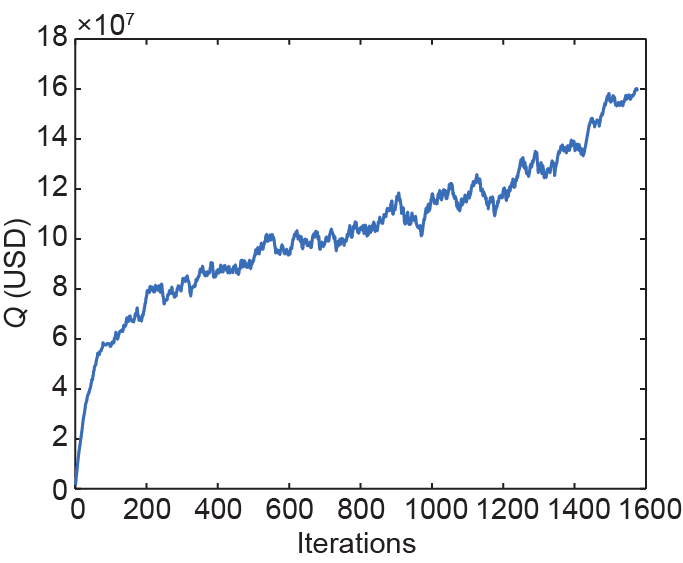
Fig. 2. Convergence of a typical state-action pair with the state i_s = 5, j_s = 7, v_s = 4, and i_a = 61.

《Fig. 3》

Fig. 3. Action values of a specific state i_s = 5, j_s = 7, and vs = 4 for all possible actions.

《Table 6》

Table 6 Levels for the settlement price and sold allowance pair (v _k–1, u_k–1 ) and levels for the time k.

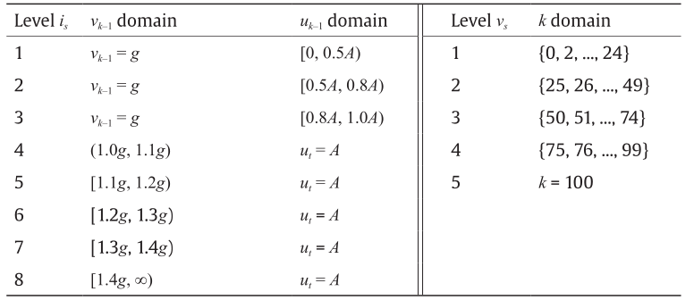
《Table 7》

Table 7 Levels for the holding account CO₂ allowances, h_k .

《4.2.Performance of the Sarsa TD algorithm》

4.2.Performance of the Sarsa TD algorithm

In this section, we show that the Sarsa TD algorithm with a time-varying flexible CO2 capture level can earn more discounted cumulative profit within the whole time horizon compared with the operation method using the fixed capture level that is specified in most of the relevant literature. The initial reserve price at time k = 0 is 12.73 USD per allowance [11]. In addition, an annual reserve price increase rate, τ, is introduced to increase the reserve price annually. This annual reserve price increase rate can simulate the development of novel technologies on carbon capture and storage. One settlement price example is shown in Fig. 4. It is observable that the settlement price is volatile during the entire time horizon (i.e., 100 quarters), and has a scheduled increase due to the annual increase rate of 5%. The same increase rate is set for the California and Quebec joint greenhouse gas auction [11,14].

《Fig. 4》

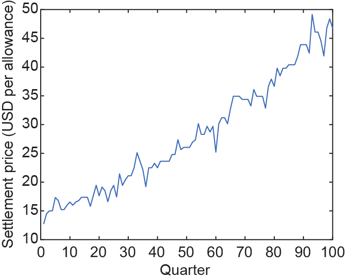
Fig.  4.  Settlement  prices  for  an  annual  increase  rate  of τ = 5% and an initial reserve price of g = 12.73 USD per allowance.

To exhibit the adaptability of the Sarsa TD algorithm, the scheduled annual increase rate, τ, is assumed to be 0%, 5%, 10%, and 15% for the CO₂  allowance reserve price. If one specific annual increase rate is fixed at τ = 0%, as shown in Fig. 5, except for the curve for the competitor (i.e., Entity 1), four reward sequences are shown for different bidding and operation strategies chosen by the decision maker of Entity 0. One bidding and operation strategy is found by the Sarsa TD algorithm with a time-varying capture level. The other strategies choose the fixed-capture-level-based operation (i.e., with the capture level set at 50%, 70%, or 90% throughout the relevant episode) and decide on the bid option with the predefined probabilities for each action under each aggregated state. Possible bid options for the fixed-capture-level-based strategy also come from the bid option set, B₀, which is the same as that of the Sarsa-based unified bidding and operation strategy. Note that the aforementioned reward sequences indicate the quarter-based profits of the power plant throughout its lifetime. By computing the discounted sum of a specific reward sequence, one can obtain the discounted cumulative profit of a specific bidding and operation strategy. Based on Fig. 5, the discounted cumulative profit with the annual reserve price increase rate, τ, of 0% can be calculated for each strategy.

《Fig. 5》

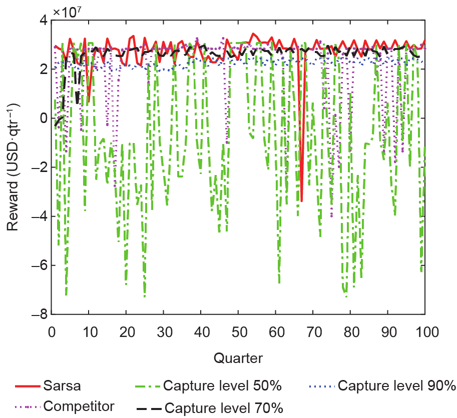
      Fig. 5. Rewards for different bidding and operation strategies with an annual increase rate of τ = 0% and the initial holding account CO₂  allowance of h₀ = 0.05 × 10⁶.

Analogously, as shown in Fig. 6–Fig. 8, one can obtain the discounted cumulative profits with the initial holding account CO₂ allowances h₀ = 0.05 × 10⁶ and with τ changing from 5% to 15%. The discounted cumulative profits for different reserve price increase rates under specific initial holding account CO₂  allowances h₀ = 0.05× 10⁶ are shown in Fig. 9.

《Fig. 6》

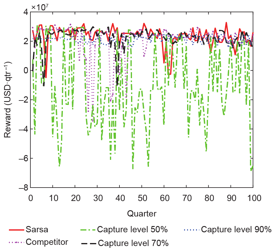
Fig. 6. Rewards for different bidding and operation strategies with an annual increase rate of τ = 5% and the initial holding account CO₂  allowance of h ₀= 0.05 × 10⁶.

《Fig. 7》

       Fig. 7. Rewards for different bidding and operation strategies with an annual increase rate of τ = 10% and the initial holding account CO₂  allowance of h₀ = 0.05 × 10⁶.

《Fig. 8》

Fig. 8. Rewards for different bidding and operation strategies with an annual increase rate of τ = 15% and the initial holding account CO₂  allowance of h₀ = 0.05 × 10⁶.

《Fig. 9》

Fig. 9. Discounted cumulative profits with the initial holding account CO₂ allowance of h₀ = 0.05 × 10⁶ and the initial reserve price g₀ = 12.73 USD per allowance.

Furthermore, the discounted cumulative profits for other initial holding account CO₂ allowances are presented in Fig. 10 and Fig. 11. It can be implied that whatever fixed capture level may be set by the decision maker using the fixed-capture-level-based method, the unified flexible operation and bidding strategy found by the Sarsa TD performs better.

《Fig. 10》

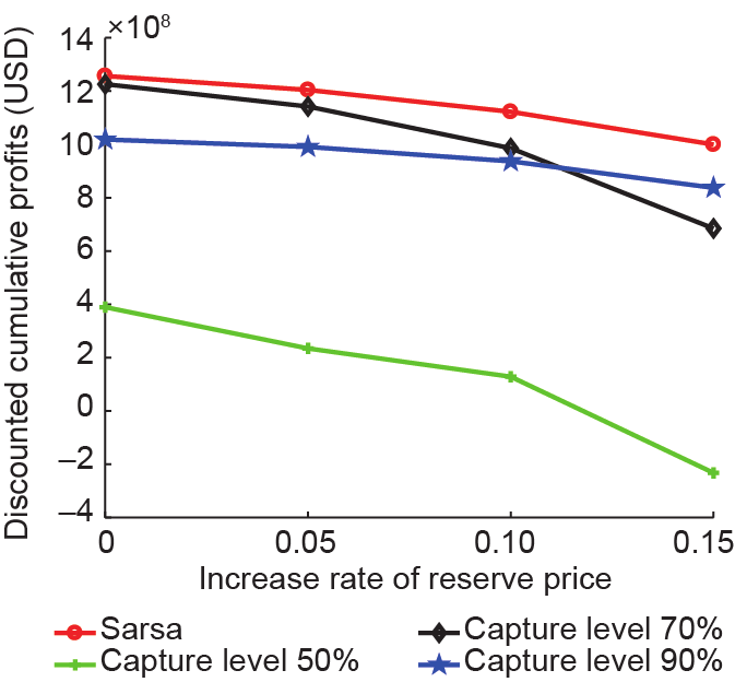
Fig. 10. Discounted cumulative profits with  the initial holding account CO₂ allowance of h₀ = 3 × 10⁶ and the initial reserve price g₀ = 12.73 USD per allowance.

《Fig. 11》

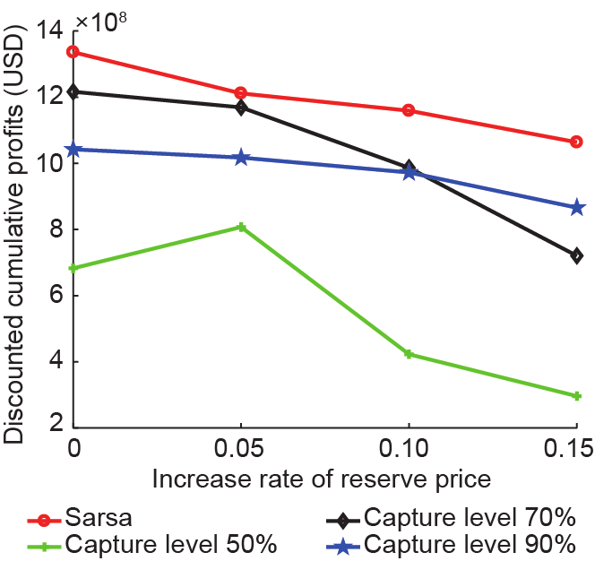
Fig. 11. Discounted cumulative profits with the initial holding account CO₂ allowance of h₀ = 5 × 10⁶ and the initial reserve price g₀ = 12.73 USD per allowance.

《4.3.Comparison with another entity in the allowance market》

4.3.Comparison with another entity in the allowance market

We consider the performance of the Sarsa TD algorithm for the decision maker compared with a competitor, Entity 1, in the same CO₂ allowance market. For this competitor, all settings of the power plant are assumed to be the same as those for Entity 0. Regarding the operation and bidding method, Entity 1 has its capture level fixed at 60% while it independently selects the bid option from B₀, the same as Entity 0. It is assumed that the bid option selection behavior of Entity 1 is approximated with the Boltzmann distribution by the decision maker of Entity 0, as follows:

where y and z are the indices of the available bidding options; n_b is the total number of bid options that is equal to 16 for the bid option set B₀; Pr(y) denotes the probability of choosing the bid option with an index of y; and ξ is the temperature of the distribution. From Eq. (33), a large ξ indicates that the selection of each possible bid option is nearly equiprobable. For simplicity, ξ = 1 in this case study. The variable ω represents the weightings for each option indexed by y or z. In our simulation, the maximum among all weightings is a constant, ω_max = n_b. It is assumed that the 13th bid option is assigned with the maximum weighting, that is, ω(y = 13) = ω_max = 16. Weightings of all the possible bidding options are decreased by 1 per index centered at y = 13. Thus, all the weightings are specified and listed as follows: 4, 5, 6, 7, 8, 9, 10, 11, 12, 13, 14, 15, 16, 15, 14, 13. With these weightings, the probability of choosing one possible bid option can be predefined in terms of Eq. (33). In practice, the decision maker can obtain either the historical bidding data of this competitor or the historical market conditions to identify weightings.

In Fig. 12 and Fig. 13, the holding account CO₂ allowances of the decision maker, hk, and those of the competitor are plotted, respectively. The discounted cumulative profits of both entities are shown in Fig. 14, which is derived with reward sequences from Fig. 5 to Fig. 8 for the decision maker applying the Sarsa TD algorithm and for the competitor. In Fig. 14, the decision maker gains more discounted cumulative rewards for different annual increase rates of the reserve price, which suggests that a better bidding and operation strategy through the Sarsa TD algorithm is applied by the decision maker than the strategy implemented by the competitor in the same CO₂ allowance market.

《Fig. 12》

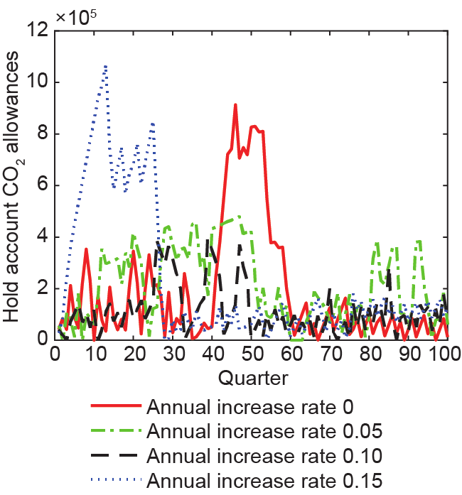
Fig. 12. Decision-maker holding account CO₂ allowances using the Sarsa TD strategy for different reserve price increase  rates.

《Fig. 13》

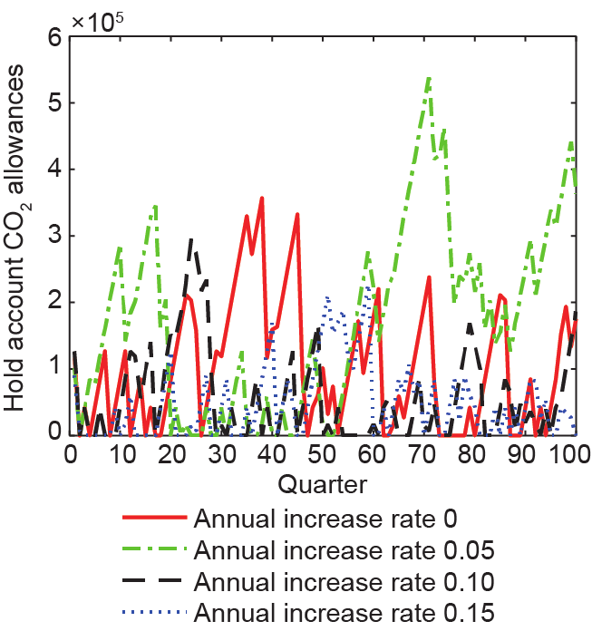
Fig. 13. Competitor holding account CO₂  allowances for different  reserve  price  increase  rates.

《Fig. 14》

Fig. 14. Discounted cumulative profits of the decision maker, Entity 0, and of Entity 1, both with the initial holding account CO₂ allowance of h0 = 0.05 × 10⁶.

《5.Conclusions》

5.Conclusions

A unified bidding and operation strategy found by the Sarsa TD algorithm  is  presented  for  a  coal-fired  power  plant  with  carbon capture. It is demonstrated that the proposed strategy, using a time-varying flexible CO₂ capture level from the capture level set and a bidding option set, is better than a fixed-capture-level-based operation with an independently designed bidding strategy. The Sarsa TD algorithm can maximize the discounted cumulative profit for the power plant under different CO₂ allowance market conditions, such as a different annual increase rate of the reserve price or different initial holding account CO₂ allowances. Furthermore, compared with another power plant with a fixed capture level and a randomly designed bidding strategy using the Boltzmann distribution, the decision maker implementing the strategy from the Sarsa TD algorithm is more competitive in the CO₂ allowance market.

《Compliance with ethics guidelines》

Compliance with ethics guidelines

Ziang Li,  Zhengtao  Ding,  and  Meihong  Wang  declare  that  they have no conflict of interest or financial conflicts to disclose.