《1. Introduction》

1. Introduction

With digitization of manufacturing currently at the forefront of a new industrial revolution, process industries are in the transition toward a smart manufacturing era, popularly called Industry 4.0 [1]. Industry 4.0 aims to create smart factories, wherein ① physical devices have virtual counterparts that are integrated with intelligent computing algorithms carrying models to mimic real processes; ② such devices are interconnected in real and virtual worlds and are connected to a centralized database; and ③ with limited human intervention, the connected devices will automate processes based on integrated decision-making using real-time information, thus driving production processes toward the optimal target values [2]. In order to materialize the aforementioned concepts of Industry 4.0, new continuously operated robotic devices have been developed in all sectors of engineering to guarantee faster transfer of reliable scientific information from first feasibility studies to pilot plants [1]. An example in chemical engineering applications is the use of automated continuous-flow microreactor systems for understanding and modeling the kinetic phenomena of chemical processes from real-time experimental data. In the study of chemical processes, automated microreactor systems with online analysis and feedback control loops for optimal experimental design have been successfully applied for ① online optimization of a performance criterion of the process, such as the percentage yield of a chemical reaction (referred to as "selfoptimization”) [3–7]; ② discrimination between competing kinetic models [8,9]; and ③ precise estimation of the parameters of a kinetic model [7,10,11].

When the aim is to identify kinetic models online—that is, during the execution of experiments—the automated microreactor system employs sequential model-based design-of-experiments (MBDoE) methods in the feedback loop for designing new experiments. In sequential MBDoE [12], data from past experiments are used to gain information (Fisher information) about the system, which is related to the uncertainty in the estimation of parameters of a candidate model structure. The past information is then used to design future experiments in such a way as to maximize the expected information or minimize the uncertainty in successive parameter estimation. This process of designing experiments for minimizing parametric uncertainty is iterated until a desirable precision on the parameter estimates is achieved. In most of the previous studies [10,11] on model identification, the optimal experimental design problem was formulated as single objective optimization problem based on some measure of the expected Fisher information matrix (FIM). In the case of steady-state processes, the maximum amount of information gained per experiment is limited by the time and cost of the experiments. In such cases, it is worth analyzing the information gained per experiment and the associated economic and operational performance through multi-objective optimal experimental design approaches. This will help to design experiments for model identification in an overall optimal way and can answer questions such as what level of information can be achieved given a certain expense or time.

A typical multi-objective optimization problem involves the determination of a set of nondominated trade-off solutions, called Pareto-optimal solutions. The set of corresponding objective vectors is called a Pareto front [13]. The methods for solving multiobjective optimization problems can generally be classified into classical and evolutionary methods. In classical methods, a solution set close to the Pareto optimal is obtained by solving the multiobjective problem as a number of single-objective optimization problems in which either all the objectives are aggregated together (weighted sum method [14]) or all the objectives except one are constrained (ε-constraint method [15]). On the other hand, evolutionary methods produce a solution set that is close to the Pareto optimal in each single run of the optimization algorithm [16]. The choice of the algorithm is mostly problem-specific and is related to a compromise between the convergence and computational time. For a more detailed description of the various algorithms and their choices, the interested reader is referred to Refs. [13,17].

Previously, in the identification of kinetic models, a multiobjective optimal experimental design approach was employed to study the trade-off between different FIM-based criteria for improving the parameter estimation problem in bioprocess systems [18]. Other applications of multi-objective optimization in optimal experimental design for model identification include the joint model-based experimental design approach [19] for simultaneously improving parameter estimation and model discrimination, and experimental design approaches for improving parameter precision and minimizing parameter correlation [20]. For highly nonlinear systems, multi-objective optimal experimental design approaches for maximizing the FIM-based metric while minimizing the model curvature have been applied to improve FIM-based model identification procedures [21]. In addition, the implementation of multi-objective optimization with efficient decision-making steps in a software interface for process simulation is discussed in Ref. [22]. This method allows the efficient design of processes with conflicting objectives through the analysis of trade-off solutions with the help of a flexible decision support facility. The advantages offered by multi-objective optimization in the optimal experimental design for model development is discussed in Ref. [23]; these scholars applied statistical design-of-experiment (DoE) methods in the most desirable regions of the Pareto front of conflicting objectives in order to design optimal experiments. Recently, a machine-learning-based multi-objective optimal experimental design approach was applied to an automated flow reactor system for selfoptimization [4]. This approach employs a Bayesian optimization algorithm to train and refine Gaussian process surrogate models that approximate the response surfaces of the objectives. In another recent study [24], a multi-objective optimal experimental design approach was applied to compare the information gained with the associated cost using different experimental design criteria for the design of carbon-labeling experiments. None of these previous works explored the possibility of applying multiobjective optimal experimental design frameworks in online model identification platforms. Such a framework will provide a flexible optimization platform that facilitates the analysis of different trade-off solutions between the information-based objective function and other conflicting objectives in each iteration of the experimental design problem, and makes it possible to select the desired trade-off solution, leading to an overall optimal scenario for model identification.

In this work, a multi-objective optimal experimental design framework is proposed to improve the efficiency of online model-identification platforms. In the framework, an optimal experimental design problem is solved as a multi-objective MBDoE (MBDoE-MO) optimization problem using the ε-constraint method [15], in which one of the objective functions (process economics) is optimized while the other (information-based objective function) is constrained by different values. The framework is applied in a simulated case study to design optimal experiments for the identification of kinetic models in automated flow reactors operated at steady state. This case study is derived from a real system of kinetic model identification for the esterification of benzoic acid (BA) with ethanol (E) in a microreactor operated at a steady state [25]. Despite being simple, experimentation in flow systems that are operated at steady state involves unnecessary material consumption [26–29], which is generally at its maximum during the most informative conditions, making the overall process economically suboptimal. The proposed multi-objective optimal experimental design framework makes it possible to overcome this limitation in kinetic studies by using an information-based objective function alongside a cost-based objective function that accounts for material consumption.

《2. Materials and methods》

2. Materials and methods

《2.1. System model》

2.1. System model

An identifiable model (i.e., a model whose parameters can be uniquely estimated from sufficient experimental data) [30] for the system of interest is represented by a set of differential and algebraic equations (DAEs) in the general form given in Eq. (1).

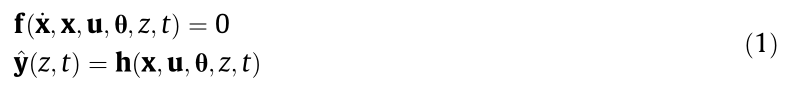
In Eq. (1), f and h are respectively the × 1 and × 1 set of equations forming the kinetic model, x is the × 1 array of state variables, is a set of derivatives of the state variables in time and space (i.e. for and , u is the ×1 array of manipulated inputs, θ is the × 1 array of model parameters, t is the time, z is the axial domain, and is the ×1 array of model predictions for the variables that are measured in the process.

The aim of the online model-identification task is to obtain the most appropriate form of Eq. (1) and to estimate the unique values of its parameter set θ using real-time data generated by automated devices. Once an appropriate model structure is identified from the data, the model identification task is reduced to the problem of estimating the parameters θ of the model as precisely as possible. This is achieved by solving the parameter estimation problem and optimal experimental design problem sequentially until a unique estimation of the parameters is confirmed by a statistical hypothesis test. The experimental design problem is solved as an optimization problem to find the optimal set of -dimensional experimental design vector that generally contains the -dimensional set of the initial conditions of the measured response variables, the -dimensional set of manipulated inputs u, the -dimensional set of the sampling times of the output variables and, potentially, the experiment duration .

《2.2. Proposed framework》

2.2. Proposed framework

A multi-objective optimal experimental design framework is proposed to carry out the experimental design problem of online model identification platforms in order to identify the set of experimental design vectors that improves the parameter estimation with minimum experimental cost. The algorithm scheme for the proposed framework is shown in Fig. 1.

《Fig. 1》

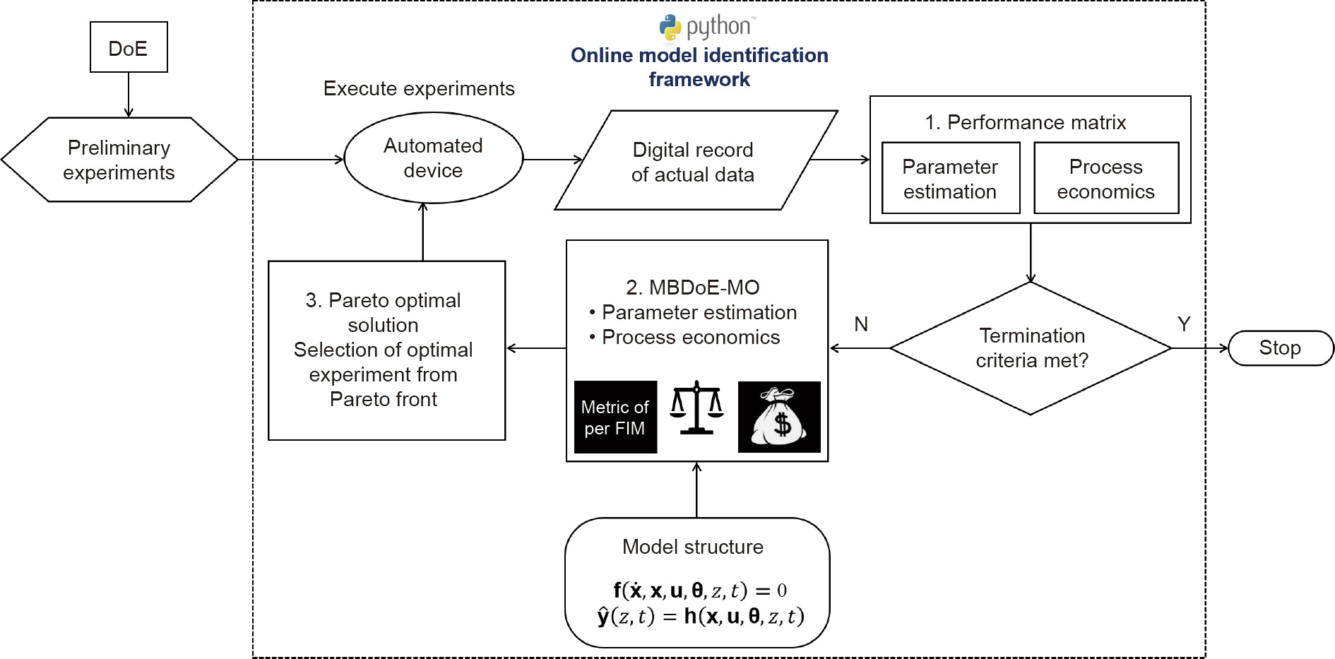
Fig. 1. Proposed framework for the online multi-objective optimal experimental design in automated model-identification platforms. The framework is used to design experiments that improve the precision of online parameter estimation with minimum experimental cost.

As shown in Fig. 1, the automated device initially performs preliminary experiments that are designed using statistical DoE methods [31]. The actual data from the preliminary experiments are stored in a digital database. From the digital record of actual data, the process performance is evaluated using predefined objective functions. The online model identification framework proposed here is based on two objectives: ① minimization of cost; and ② maximization of expected information. The process performance is evaluated during each sequence of the experimental design by calculating the experimental cost and the confidence region of the model parameters. This step is illustrated in Block 1 (performance matrix) in Fig. 1. Future experiments are designed to identify the conditions corresponding to trade-off solutions with respect to the two objectives. The trade-off conditions are obtained by solving the experimental design problem as a multi-objective optimization problem for minimizing cost and maximizing information, as represented by Block 2 in Fig. 1. In the next step (Block 3 in Fig. 1), the appropriate condition for the next experiment is selected from the generated trade-off solutions and executed automatically. The entire sequence of operations is performed online and iterates until a termination criterion is met. Termination criteria are decided by the user. Common termination criteria include ① reaching the allowed experimental budget or ② a predefined threshold value for the primary objective of the study. In the present work, criterion ① is chosen as the termination criterion. The whole framework is implemented in Python [32] and operates as an independent module with a single function call. The multiobjective optimal experimental design framework constitutes the core part of the implemented algorithm; details on its formulation are explained in the following sections. The optimal experimental design problems for MBDoE methods for improving parameter estimation (MBDoE-PE) and MBDoE method for minimizing exper imental cost (MBDoE-cost) are discussed first, which is then followed by the formulation of MBDoE-MO and its solution method.

《2.3. MBDoE-PE》

2.3. MBDoE-PE

The FIM, whose inverse provides an estimate of the lower bound of parameter variance–covariance by the Cramer–Rao inequality [33,34], has been commonly used to define the objective function in optimal experimental designs for improving parameter precision [35]. Conventional MBDoE-PE are formulated as an optimization problem of the form:

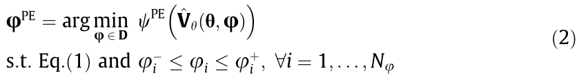
In Eq. (2), refers to some measure of the predicted parameter variance–covariance matrix , which is minimized to obtain the optimal experimental design vector which is an array with the dimensions corresponding to the N designed experiments. Commonly used choices for include the trace, eigenvalue, or determinant of the parameter variance–covariance matrix, which respectively form the alphabetic optimal design criteria called A-, E-, and D-optimal designs [36]. In the present study, the maximum eigenvalue of the parameter variance–covariance matrix was chosen as the metric of parametric uncertainty, and the E-optimal MBDoE for improving parameter precision was formulated by minimizing this objective function. The constraints of the optimization problem are the model equations and the dimensional bounds on the design variables that are allowed to vary within the design space D, defining the operational range for these variables. The predicted parameter variance–covariance matrix in Eq. (2) is calculated from the observed FIM according to Eq. (3).

In Eq. (3), represents the observed FIM obtained from the performed experiment, and the summation represents the total observed information from all previous n experiments. Similarly, represents the expected FIM for the experiment to be designed, and the summation provides the total predicted information contained in N experiments to be designed. The observed FIM is evaluated at the maximum likelihood estimate [34] of model parameters. The expected FIM for the designed experiment is calculated using Eq. (4), as given below.

In Eq. (4),  denotes the standard deviation of the measurement error associated with the measurement of the response variable in the   sampling of the jth experiment, and  denotes the  ×1 dimensional column vector of the first derivatives of the lth response variable in the  sampling with respect to the model parameters, and represents the first-order sensitivities of the responses with respect to the parameter values,  is the transpose of .

《2.4. MBDoE-cost》

2.4. MBDoE-cost

To improve the process economics associated with performing the experiments, MBDoE-cost is formulated as follows:

where  represents the cost function associated with the execution of experiment, the summation is the total cost of performing N experiments, and represents the set of constant parameters in the cost function. The definition of the optimization decision variables and the constraints related to the model equations and design space remain the same as in the MBDoE-PE.

《2.5. Formulation of the multi-objective optimal experimental design problem》

2.5. Formulation of the multi-objective optimal experimental design problem

The MBDoE-MO for improving the precision of the parameter estimation with minimum experimental cost is solved by the ε-constraint method, in which the cost function is minimized by restricting the FIM-based objective function within different values of ε. The MBDoE-MO optimization problem is formulated as:

The unique solution   of the MBDoE-MO optimization problem stated in Eq. (6) is Pareto optimal for any given N_k -dimensional upper bound vector: .  It is possible to find different Pareto-optimal solutions using different ε values. Ideally, the ε vector must be chosen such that each ε lies between the minimum and maximum values of the objective function that is restricted to constraints. This means that  should respectively be the minimum and maximum values of the restricted objective function, which is the maximum eigenvalue of the parameter variance–covariance matrix  in the present problem. Thus, the minimum value of e, that is, ε = ε₁, is the value of in the solution of the MBDoE for improving the parameter estimation, that is,  and the maximum value of ε, that is, ε = is the value of wPE in the solution of the MBDoE for improving process economics, that is, .

《2.6. Selection of the Pareto-optimal solutions》

2.6. Selection of the Pareto-optimal solutions

The solution vector obtained by solving Eq. (6) is an array, when N number of experiments are designed by solving the multi-objective optimization problem. In order to navigate within the online model-identification framework, it is necessary to select one solution from as the condition for the next experiment. For this purpose, an algorithm based on a measure called the trade-off index (referred to herein as the "TO-index”)—which indicates the distance of any point on the Pareto curve from the point that corresponds to the minimum value of two objective functions if the functions were not mutually conflicting—is proposed to analyze the set of optimal trade-off solutions and to select the desired trade-off solution for the next experiment. The TO-index is evaluated using the normalized values of the objective functions denoted by contained in the normalized objective vectors . The objective functions are normalized using the formula given in Eq. (7).

In Eq. (7), obj refers to PE or cost. The two-step algorithm for calculating the TO-index of each of the Pareto-optimal solutions is given below.

《2.7. Algorithm for calculating the TO-index》

2.7. Algorithm for calculating the TO-index

(1) Normalize the two N_k-dimensional objective vectors to form the normalized objective vectors  corresponding to the trade-off solutions, such that all values of  and  lie between 0 and 1.

(2) The TO-index for each of the trade-off points in the objective space is evaluated as:

where ω₁ and ω₂ are weight factor 1 and weight factor 2, respectively, used to select trade-off solutions by acting on .

(3) The Pareto-optimal solution with the smallest value of the TO-index is chosen as the condition for the next set of experiments.

The whole solution procedure described above for solving a multi-objective optimal experimental design problem in each sequence of the optimal experimental design is illustrated in Fig. 2.

《Fig. 2》

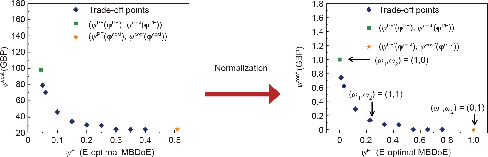
Fig. 2. Illustration of the decision-making step in the proposed multi-objective optimal experimental design framework. The set of trade-off points in the objective space obtained from the ε-constraint method are shown in the left panel. From the normalized trade-off points (shown in the right panel), appropriate conditions for the next experiment are obtained using different values of the weight factors ω₁ and ω₂; this facilitates a desired degree of trade-off solution to be chosen according to the user’s interest.

The method is developed on the basis of geometrical interpretation of the Pareto front. As shown in Fig. 2, when the Pareto objective vectors are normalized, the worst trade-off points for the objective functions, which are mutually conflicting, can be represented by the coordinates (0,1) and (1,0). The distance between any point on the Pareto curve and a minimum point (0,0), which would have become the optimal point if the functions were not mutually conflicting, is indicated by the value of the TO-index. In the decision-making step involved in each run of the MBDoEMO optimization problem, the algorithm selects the Paretooptimal point from the set of nondominated trade-off points with the lowest value of the TO-index. The next experiment is carried out under the conditions corresponding to the selected Pareto point. When the weight factors ω₁ and ω₂ in Eq. (8) are set to 1, the algorithm selects the Pareto-optimal solution by giving equal importance to both objective functions. However, in each sequence of the multi-objective optimal experimental design problem, it is also possible to select the Pareto-optimal point with the desired degree of trade-off between the objective functions. This is achieved by changing the value of one of the weights within the closed interval [0, 1], while keeping the other equal to 1, thus providing a flexible platform to choose the desired trade-off solution at any sequence of the operation. For example, when setting the value of ω₁ = 0, while keeping ω₂ = 1 in Eq. (8), the algorithm becomes a single-objective one in terms of the minimization of cost (MBDoE-cost), and selects the condition with minimum cost as the condition for the next experiment. Similarly, when ω₂ is set to 0, while keeping ω₁ at 1 in Eq. (8), the algorithm converges to the MBDoE-PE and proceeds with the most informative conditions regardless of experimental cost. In cases when ω₁ = 0 and ω₂ = 1, or ω₁ = 1 and ω₂ = 0, that is, when the decision-making process becomes a single-objective one, if there are several possible trade-off solutions with the same TO-index value, then the algorithm selects the solution that is also a minimum for the objective function whose weight is set to 0. In order to ensure an efficient local search routine in the optimization algorithm, a stochastic initialization step using Latin hypercube sampling was included in all the optimal experimental design problems solved in the framework, and no numerical issues related to convergence were observed. The impact of initialization and upper bound constraints on the distribution and convergence of Pareto-optimal solutions is discussed in the Supplementary data. The computational time required for the algorithm to solve each optimization problem is on the order of seconds. The scientific Python (SciPy) package was used for the integration of the system of ordinary differential equations in the model (using the odeint tool) and for solving optimization problems (parameter estimation and experimental design). All the array operations were performed using the NumPy library. The optimization problems of parameter estimation and optimal experimental design were solved using the Nelder–Mead and sequential least squares programming methods, respectively.

《2.8. Case study》

2.8. Case study

The proposed framework for multi-objective optimal experimental design is applied to a simulated case study related to the identification of a kinetic model for the esterification of BA with E in a microreactor. The kinetic model, objectives, modeling assumptions, and methods used in the case study are described in the following subsections.

2.8.1. Kinetic model

The esterification reaction between BA with E produces ethyl benzoate (EB) as the main product, with water (W) as a side product [37], and can be represented as follows:

The reaction is assumed to take place in a microreactor operated under steady-state and isothermal conditions. It is assumed that the microreactor behaves as an ideal plug flow reactor due to a large axial to radial dimension ratio, making the radial diffusion fast. The reactor length is assumed to be 2 m. The process is modeled as a first-order reaction with respect to BA and forms a set of DAEs given by the equation.

In Eq. (10), is the concentration of the ith species, is the axial coordinate along the reactor length, is the axial velocity of the reaction mixture which is defined as the ratio of volumetric flowrate of reaction mixture and cross-sectional area of reactor is the stoichiometric coefficient of the species, and k is the reaction rate constant. The Arrhenius equation is written in the reparametrized form given in Eq. (10), where T is the reaction temperature and R is the ideal gas constant. This form of reparametrization reduces the parameter correlation and improves the parameter estimation and the quality of the statistical tests [38]. The parameters of the Arrhenius equation—namely, the activation energy E_a and preexponential factor A—form the set of model parameters that need to be estimated, and are estimated as ln A and E_a× 10^-4 , respectively; that is, .

2.8.2. Objectives, assumptions, and methods

The objective of the case study is to estimate the kinetic parameters precisely by minimizing experimental cost. For this purpose, the proposed multi-objective optimal experimental design framework is applied to design an optimal set of experiments. As the reactor is operated under steady-state conditions, for each experiment, the measured values correspond to the steady-state concentrations of BA and EB sampled at the reactor outlet. Thus, each experiment involves one measurement sample denoted by . It is assumed that the measurement errors associated with  are normally distributed random variables with 0 mean and standard deviations of 0.03 and 0.01 mol·L^-1 , respectively; that is, the standard deviation vector =[0.03 0.01]^T.

The experimental design space D is a three-dimensional region bounded by the ranges of the operating conditions of the experimental design variables, which are the reaction temperature T (343–423 K), inlet stream flowrate (7.5–30 μL·min^-1 ), and inlet concentration of BA(0.9–1.55 mol·L^-1 ). When called upon, the experimental design problem identifies the optimum conditions within the design space D for the future experiments by solving either Eq. (2) or Eq. (6), depending on whether MBDoE-PE or MBDoE-MO is used. It is assumed that a maximum number of seven experiments is allowed in a campaign. The two preliminary experiments are designed using a factorial DoE method. This is to ensure that before starting the application of MBDoE, an estimate of the parameter is available and a minimum threshold on information is guaranteed. The conditions of the two preliminary experiments are T = 413 K, = 20 μL·min^-1 , = 1.5 mol·L^-1 and T = 393 K, = 20 μL·min^-1 , = 1.5 mol·L^-1 respectively. The online multi-objective optimal experimental design is then employed to design the next five experiments sequentially in an automated manner in a loop that iterates five times.

In real systems that are operated automatically for online model identification, if the reaction mixture analysis is not sufficiently quick, delays are introduced in accessing the information from the system after sampling. This delay can be overcome to an appreciable extent by overlapping the experiments such that every time the sample from the running experiment is sent to the analytical instrument, a new experiment is available to start. To incorporate this concept in the present problem, the first experimental design problem is solved for designing two experiments (i.e., N = 2 in Eqs. (3), (5), and (6) in the first sequence of the experimental design problem), so that when the steady-state concentrations from the first designed experiment are sampled, the second experiment is ready to start. In other words, this means that although five experiments are designed in sequence, only four optimal experimental design problems are solved. In order to perform the simulation study, in-silico measurements are generated by integrating the kinetic model in Eq. (10) using the parameter values of θ^*=[19.99 7.85]^T . Here, it is assumed that the parameter set θ^* represents the true value of the model parameters; the corresponding values of the pre-exponential factor A and the activation energy E_a are 8.0 ×10⁶ s^-1 and 7.85 ×10⁴ J·mol^-1 , respectively.

2.8.3. Evaluation of cost function

In the kinetic study using flow reactors operated under steadystate conditions, the reaction mixture is flushed out until a steady state is achieved, and only the measurements made at a steady state are used for fitting the model and estimating the parameters. Thus, to evaluate the cost, the amount of material flushed out until a steady state is achieved must be determined, which in turn requires an estimate of the time needed to reach the steady state. The cost function for the flow reactor system was formulated by accounting for the cost of the materials flushed out in any experiment j as given by:

.

In Eq. (11), is the calculated time to reach the steady state for experiment j, the product   represents the moles of BA in the volume flushed up to time  respectively denote the flowrate and inlet concentration of BA, and unit cost is the cost of 1 mol of BA, which is assumed to be 59 GBP (about 74 USD).

In order to calculate the approximate time to reach steady state for each experiment, an offline method using time series data (i.e., data collected at regular intervals during the transient period) generated during a previous campaign of steady-state experiments for the esterification reaction (carried out in a real flow reactor system identical to the simulated system) was employed. The previous campaign consisted of factorial experiments with the same experimental design variables and ranges described in the previous section. All the experiments in the campaign were run for 1 h in order to guarantee steady-state operation. During this time, samples were taken every 7 min, yielding 7–8 samples for each experiment. This process resulted in time series data. An expression for the time needed to reach a steady state in terms of the experimental design variables was obtained from the time series data through the following steps:

Step 1: Estimation of the time to reach a steady state. In this step, the approximate time to reach a steady state for each experiment was calculated from the time series data. An algorithm based on a fixed window (window size = 3 in the present study) moving average method was used to calculate the standard deviation of the measurement error in the time series data. The fixed window size corresponds to the number of consecutive samples used to calculate the standard deviation of error. If the calculated value of the standard deviation of error is less than the assumed standard deviation of the measurement error, then it is concluded that the system has reached a steady state and the algorithm stops. For each experiment, the algorithm becomes active after a residence time equivalent to 1.5 times the combined volume of the reactor and the analysis loop divided by the volumetric flowrate, which is a recommended rule of thumb for achieving a steadystate condition [26].

Step 2: Development of empirical model for the time to reach a steady state. In this step, an empirical model with the steady-state time as the response variable and the experimental conditions as the factors was developed by fitting the data generated in Step 1. It is assumed that the inlet concentration has a negligible effect on the time required to reach a steady state. A polynomial function was used to describe the relationship between the time needed to reach a steady state and the experimental conditions, which is given in Eq. (12).

In Eq. (12), represents the time to reach a steady state for the experiment with temperature and flowrate is the temperature difference between the and (j–1)th experiment, V is the total volume of the reactor and the analysis loop (i.e., the section between the reactor outlet and the HPLC sampling valve), n_past is the number of steady-state experiments belonging to a previous campaign of experiments, and and are parameters of the empirical model and are related to the length of time that the system would require to reach the steady state after a change in temperature or flowrate, respectively. The parameters were estimated by fitting the polynomial model to the data generated in Step 1 using the maximum likelihood estimation method [34]. The estimated value for the parameter set is =[18:38, 1:83]^T .

《3. Results and discussion》

3. Results and discussion

Two experimental design campaigns are compared below.

(1) MBDoE-PE: This is an optimal experimental design for improving the parameter estimation by minimizing the uncertainty of the estimated values of the model parameters.

(2) MBDoE-MO: This is an MBDoE for designing multi-objective optimal experiments to improve the parameter estimation with a simultaneous reduction of experimental cost.

The results are reported in Section 3.1 (MBDoE-PE) and Section 3.2 (MBDoE-MO).

《3.1. MBDoE-PE: An MBDoE for improving parameter estimation》

3.1. MBDoE-PE: An MBDoE for improving parameter estimation

The designed experimental conditions and the corresponding value of the parameter estimates with a 95% confidence interval (CI) in each sequence of the execution of the designed experiments are reported in Table 1. The approach involved the solution of four parameter estimation and experimental design problems (Eq. (2)) sequentially in the online platform. As shown in Table 1, the parameter estimates quickly converged to the assumed true value of the model parameters θ* = [19.99,7.85]^T after the two preliminary experiments. This shows the close agreement of the selected model to the data. However, the 95% CI, which is a measure of the variance of parameter estimates [34], suggest that the uncertainty in parameter estimation is large at the beginning. In order to improve the confidence in the estimated parameter values, five more experiments with the objective of minimizing the uncertainty in the parameter estimates are designed online. In the first experimental design problem, two experiments are designed simultaneously using the parameter estimates obtained from the preliminary factorial experiments. The remaining three experiments are then designed each time a new experiment is executed and the parameter estimates are updated. The designed experiments and the corresponding value of parameter estimates with 95% CI are given in Table 1.

《Table 1》

Table 1 Results of the online MBDoE-PE campaign, including experimental settings, posterior statistics on parameter estimates, and experimental cost for each designed experiment.

Conc.: concentration.

It is clear from the results that the uncertainty in parameter estimation has been greatly reduced over the course of the designed experiments. The experimental cost for the preliminary experiments and for each of the designed experiments for comparing the conventional MBDoE to improve the parameter estimation with the proposed MBDoE-MO have been calculated and are reported in Table 1.

《3.2. MBDoE-MO: An MBDoE for improving multi-objective parameter estimation while minimizing cost》

3.2. MBDoE-MO: An MBDoE for improving multi-objective parameter estimation while minimizing cost

In the MBDoE-MO, experiments are designed to improve the parameter estimation with minimum experimental cost. Similar to the MBDoE-PE, this approach involves solving four parameter estimation and optimal experimental design problems (Eq. (6)) online to design five optimal experiments. In the first experimental design problems, two experiments are designed using the parameter updates obtained from preliminary factorial experiments. In the subsequent experimental design problems, one experiment was designed each time the parameter estimates were updated from a new experiment. A set of seven trade-off solutions corresponding to seven different upper bound values of ε (i.e., setting N_k = 7) was obtained during each experimental design problem, from which a Pareto-optimal point was chosen by the decisionmaker. The set of trade-off points and the selected point in each experimental design problem are illustrated in Fig. 3.

《Fig. 3》

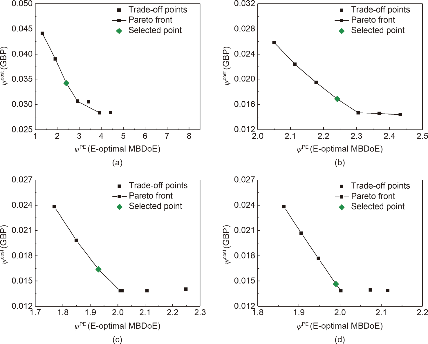
Fig. 3. MBDoE-MO procedure for the design of five experiments. (a) Design of the first two experiments of the campaign, where each point of the curve corresponds to two optimal experimental conditions; (b) MBDoE-MO procedure for the design of the third experiment; (c) MBDoE-MO procedure for the design of the fourth experiment; (d) MBDoE-MO procedure for the design of the fifth experiment of the campaign. The black squares are the different trade-off points (nondominated/dominated) corresponding to different values of the upper bound variable ε. The green diamond is the selected point from the set of trade-off points, such that the solution at this point is chosen as the conditions for the next set of experiments. In all the cases, the selected point is Pareto optimal.

As indicated in the figure, a multi-objective optimal experimental design problem involves the solution of N_k (here, N_k = 7) optimization problems corresponding to N_k different values of the upper bound variable ε; this was solved online in the proposed platform. The appropriate solution for the next experiment is selected from the set of trade-off solutions by assigning appropriate values to the weight factors ω₁ and ω₂ (see Section 2.5). In the present problem, both ω₁ and ω₂ were set at 1 in Eq. (8) in order to select the best trade-off solution (giving equal importance to both objectives). By assigning appropriate values to the weights, it is possible to select Pareto-optimal solutions according to the required degree of trade-off between the two objective functions. The results of the MBDoE-MO are summarized in Table 2. As shown in the table, a significant reduction of the experiment cost has been achieved with only a slightly lower precision of parameter estimation, compared with the results of the MBDoE-PE campaign.

《Table 2 》

Table 2 Results of the online MBDoE-MO campaign. Optimal settings of experiments, posterior statistics on parameter estimates, and experimental cost for each designed experiment are shown.

《3.3. Comparison of results》

3.3. Comparison of results

The results of both the campaigns of experimental design (MBDoE-PE and MBDoE-MO) are compared. In terms of precision in the estimation of the model parameters, both the MBDoE-PE and the MBDoE-MO improve the estimation of the model parameters in the successive experimental design problems. This is illustrated in terms of the CIs of the parameter estimates in Fig. 4 and using the parameter statistics (95% t-value) in Fig. 5(a). The CI for any parameter estimate with significance level can be computed as:

In Eq. (13),  is the two-tailed t-value of a t-distribution with  degrees of freedom and significance, and  represents the standard deviation of the  parameter estimate . The t-value for any parameter estimate is computed as the ratio between the parameter estimate and the CI:

The reference t-value is the t-value of a t-distribution with  degrees of freedom and significance; that is, . For any parameter estimate, a t-value higher than he reference t-value indicates a statistically precise estimation of that parameter. As expected, the MBDoE-PE produces a more precise estimation of both model parameters in comparison with the MBDoE-MO. This is evident from the width of the CIs for the parameter estimates shown in Fig. 4, which indicates the margin of error around the estimated value. As shown in Fig. 4, in the MBDoE-PE campaign, both parameters have approached to the true values with a minimum uncertainty defined by the narrow CI. The small fluctuations of parameter estimates around the true value can be attributed to the random noise added in the simulated experiments. Compared to the MBDoE-PE campaign, in the MBDoE-MO campaign, the parameter estimates are relatively far from the true values and the CIs are wider. The higher t-values of the parameter estimates obtained in the MBDoE-PE campaign compared with the MBDoE-MO campaign also indicate that the parameters are estimated more precisely in the MBDoE-PE campaign. This is shown in Fig. 5(a). In contrast, the information-rich experiments designed by the MBDoE-PE are more expensive than those designed by the MBDoE-MO. A comparison of the cost of each of the experiments designed through both approaches is given in Fig. 5(b).

《Fig. 4》

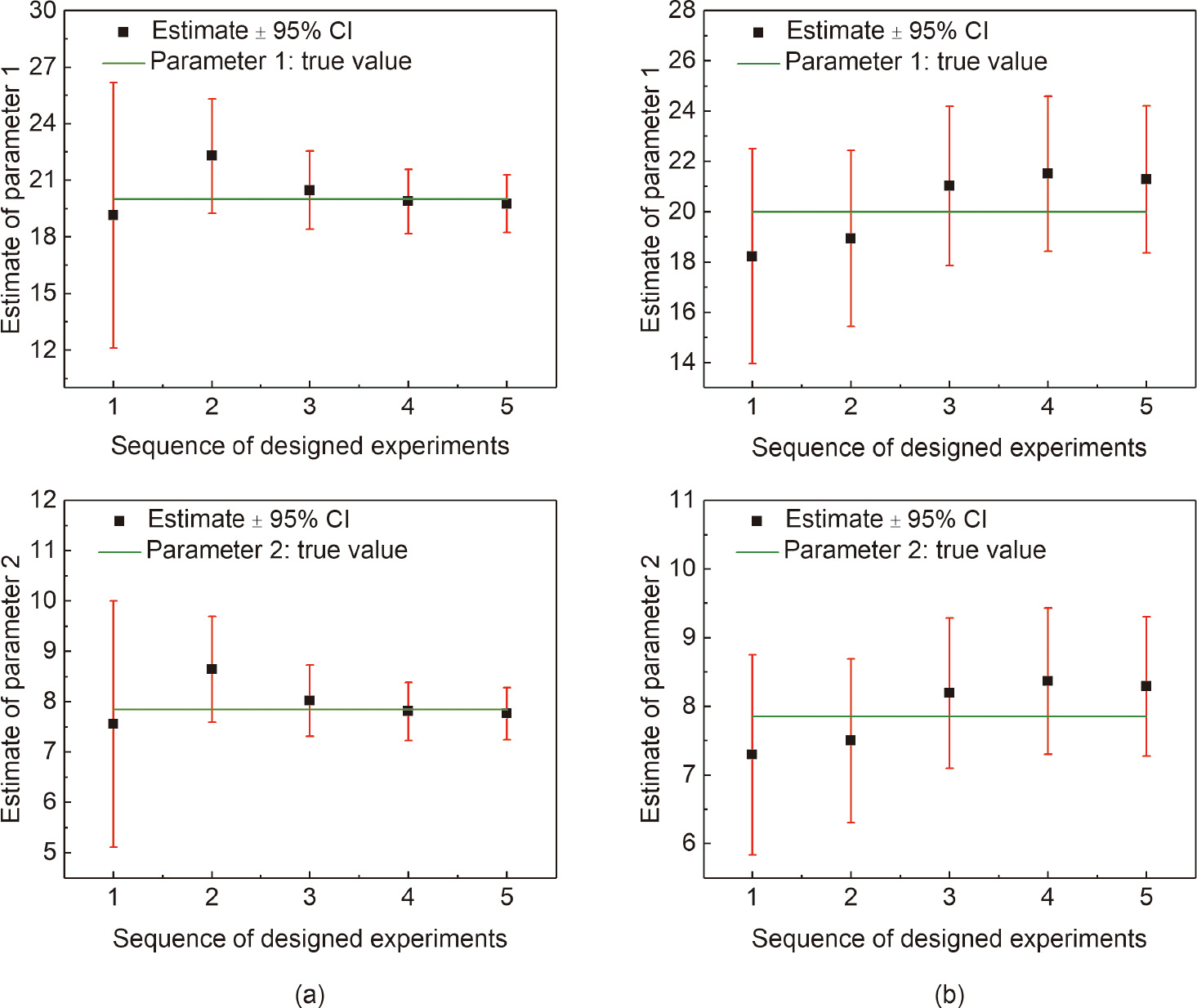
Fig. 4. Parameter estimates with 95% CIs for the model parameters in each experiment of (a) the MBDoE-PE campaign and (b) the MBDoE-MO campaign.

《Fig. 5》

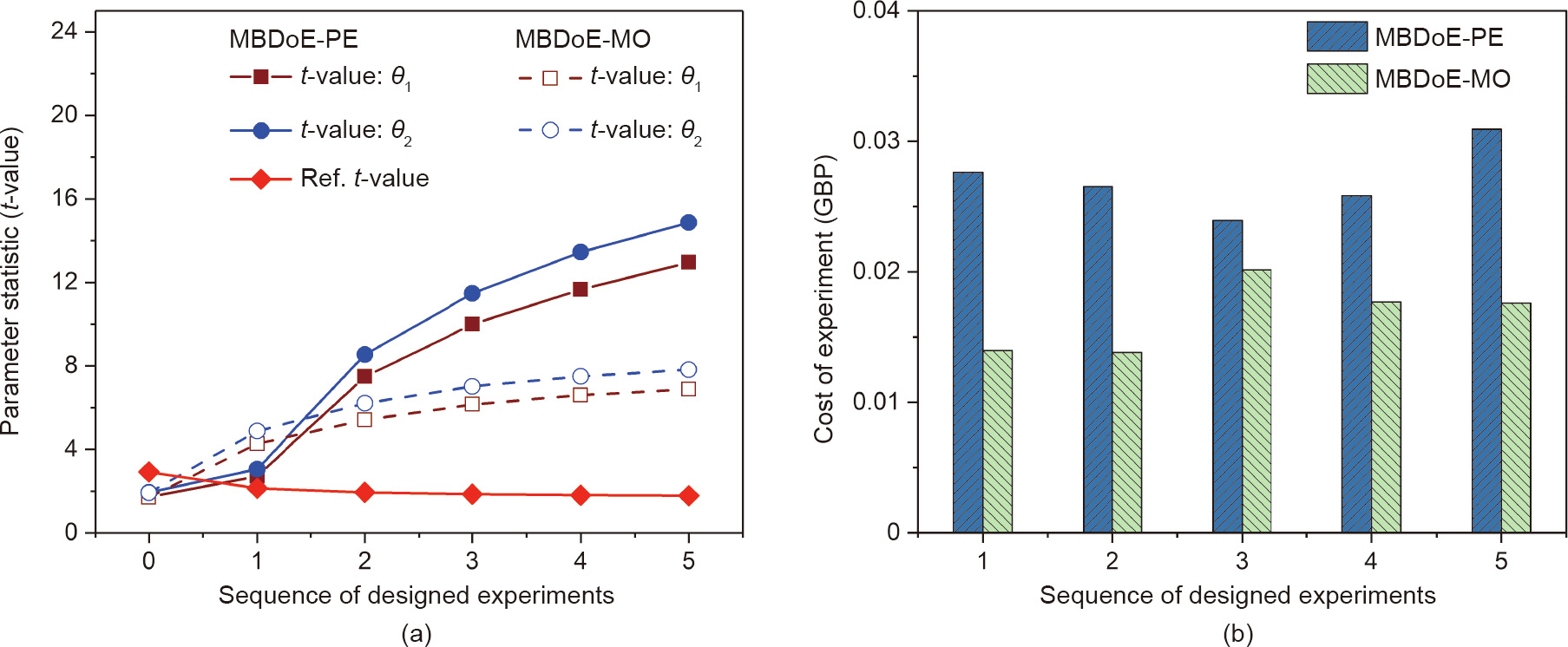
Fig. 5. A comparison of the results from the MBDoE-MO and MBDoE-PE campaigns in terms of (a) parameter statistic (95% t-value) and (b) the cost of materials in each experiment. In (a), a t-value greater than the reference t-value indicates a precise estimation of the model parameter. A higher t-value indicates more precise estimation.

By analyzing Figs. 4 and 5, it is clear that in situations of critical constraints on cost, the multi-objective optimal experimental design framework can provide the best trade-off solutions with respect to improving the parameter estimation and minimizing cost. The profiles of the experimental design variables (temperature, flowrate, and inlet concentration) in the designed experiments by both approaches are compared in Fig. 6. The differences in the experimental conditions of the designed experiments by both approaches are more apparent in terms of the flowrate and reactant (BA) concentration. This is due to the fact that the amount of reagent used is directly related to the inlet concentration, whereas the flowrate is the most significant factor affecting the time required to reach a steady state. The profiles of the reaction temperature and flowrate follow a similar trend in the MBDoE-PE campaign, such that the combinations of high temperature (T ≈140 °C) and low residence time (high flowrate; f ≈17 μL·min^-1 ) as well as low temperature (T ≈ 115 °C) and high residence time (low flowrate; f ≈ 7.5 μL·min^-1 ) appear to be favorable conditions to gain information about the reaction system. In the case of the MBDoE-MO campaign, the optimal conditions shift to a high flowrate and low concentration in order to minimize the material consumption.

《Fig. 6》

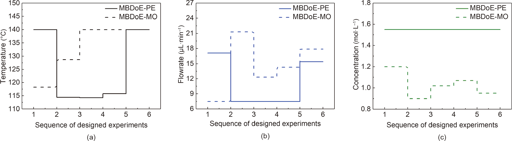
Fig. 6. A comparison of the optimal sequence of the experiments designed using the MBDoE-PE and MBDoE-MO methods. (a) Optimal temperature profiles; (b) optimal flowrate profiles; (c) optimal inlet BA concentration profiles for both MBDoE-PE (solid lines) and MBDoE-MO (dash lines).

《4. Conclusion》

4. Conclusion

The emergence of robotic devices with real-time data-based feedback loops provides a suitable environment for the online modeling and optimization of chemical processes. Optimal experimental design can play a significant role in such modeling and optimization, since it acts as an approach to plan future process conditions based on current data and desired objectives. When the optimal experimental design problem involves mutually conflicting objectives, a fair compromise can represent the best solution. In this work, a framework was proposed for online multi-objective optimal experimental design that makes it possible to find the best trade-off solutions for designing experiments when the process is subjected to multiple constraints. A solution strategy composed of a decision-making step is proposed to solve the multi-objective optimization problem online. This strategy, which uses a FIM-based metric to analyze the degree of trade-off solutions, makes it possible to select the desired Pareto-optimal point from the vector of trade-off solutions as the condition for the next experiment. The benefits of the application of this framework were demonstrated using a simulated case study on the identification of a kinetic model for the BA esterification. The results from the case study suggest that optimal experimental design using the MBDoEMO represents an improved way of conducting reaction kinetic studies in flow systems operated under steady-state conditions. This approach makes it possible to identify the best trade-off conditions to improve the information gained from the reaction system, while minimizing the cost of the materials consumed. This framework was implemented as a general function in Python, and can be extended to a large variety of real online multiobjective optimization problems.

《Acknowledgements》

Acknowledgements

This work was financially supported by the PhD scholarship awarded to A. Pankajakshan from the Department of Chemical Engineering, University College London.

《Compliance with ethics guidelines》

Compliance with ethics guidelines

Arun Pankajakshan, Conor Waldron, Marco Quaglio, Asterios Gavriilidis, and Federico Galvanin declare that they have no conflicts of interest or financial conflicts to disclose.

《Nomenclature》

Nomenclature

Latin Symbols

A pre-exponential factor

concentration of species i

 concentration of species i at the reactor inlet

 concentration of species i at the reactor outlet

E_a activation energy

volumetric flowrate

k kinetic constant

n number of designed experiments already performed

N number of experiments designed in one sequence of MBDoE methods

 number of differential and algebraic equations constituting the model

number of upper bound variable in one sequence of MBDoE-MO optimization problem

 number of manipulated inputs

 number of state variables

 number of measured variables

 number of design variables

 number of model parameters

 number of sampling points

R ideal gas constant

t time

T reaction temperature

v flow velocity along the axial coordinate of reactor

V volume of reactor

z axial domain

Matrices and vectors

D dimensional experimental design space that bounds the admissible range of values of design variables

f array of functions in kinetic model

h set of relations between the measured response variables   and the state variables 

i observed Fisher information matrix obtained from the   performed experiment ×

 expected Fisher information matrix for the design of  experiment ×

 array of sampling times  × 1

u array of manipulated control inputs ×1

 parameter variance–covariance matrix  ×

x array of state variables × 1

y array of measured output variables × 1

array of initial conditions of the measured response variables × 1

 array of model predictions of the measured output variables × 1

θ array of model parameters × 1

 array of true value of model parameters × 1

ε upper bound vector for MBDoE-MO optimization problem × 1

 experimental design vector × 1

 optimal experimental design vector for MBDoE-cost problem N ×

 optimal experimental design vector for MBDoE-PE problem N ×

 optimal experimental design vector for MBDoE-MO optimization problem × N ×

 normalized objective vector from MBDoE-cost problem ×1

 normalized objective vector for MBDoE-PE problem ×1

Greek symbols

 ith model parameter

 maximum likelihood estimate of the ith model parameter

 stoichiometric coefficient of the ith species

 upper bound variable in MBDoE-MO optimization problem

 time to reach the steady state in ith experiment

gradient operator

 weight factor 1, used to select trade-off solutions by  acting on 

 weight factor 2, used to select trade-off solutions by acting on 

 parameters of empirical model for estimating time to reach steady state

  objective function for MBDoE-PE problem

 objective function for MBDoE-cost problem

 normalized value of objective function for MBDoE-PE problem

 normalized value of objective function for MBDoE-cost problem

Acronyms

BA benzoic acid

DAE differential and algebraic equation

DoE design of experiments

EB ethyl benzoate

FIM Fisher information matrix

MBDoE model-based design of experiments

MO multi-objective

PE parameter estimation

《Appendix A. Supplementary data》

Appendix A. Supplementary data

Supplementary data to this article can be found online at https://doi.org/10.1016/j.eng.2019.10.003.