《1. Introduction》

1. Introduction

Recent studies have shown that complete gate-to-gate guidance of each flight is required for efficient operations and to meet the needs of the ever-increasing aircraft and passenger traffic at airports [1,2]. This complete guidance is called four-dimensional trajectory (4DT) guidance. 4DT is the spatiotemporal navigation of aircraft from the departure gate to the runway and vice versa (including the taxiing and pushback paths) [3]. The 4DT guidance system not only provides opportunities for optimizing the various stages of ground movement, but also coordinates the movements of a fleet of aircraft. Indeed, the 4DT guidance system has the potential to reduce taxi delays by as much as 55% [4]. It is thus not surprising that many air traffic managers are currently investigating the increased digitalization of airports, including new ground decision support and navigation technologies, in order to cope with congestion and improve resilience at airports [1]. With the number of passengers set to increase to 1.5 times the published 2012 levels by 2035 [1,5], there is now an even greater urgency to implement these 4DT algorithms in order to meet the everchallenging task of managing aircraft ground movements at various airports. Furthermore, aircraft emissions, which account for 3% of global greenhouse emissions [5,6], provide a significant motivation for ground movement optimization.

A plethora of studies have been carried out to investigate the feasibility of airport ground decision support and navigation systems [7–10]. These studies can be broadly classified into two categories. The first category includes algorithms that address the routing and scheduling of airport ground operations. Therefore, such studies focus more on airport-wide operations than on specific aircraft. Algorithms in this category mostly address the minimization of taxi time [4,11] and do not actively or directly optimize fuel efficiency and related emissions. A few exceptions, such as the active routing and scheduling algorithm [5,12], consider fuel consumption and emissions directly. However, the calculation is based on simplified equations of aircraft motion and fuel and emissions models. As a result, the generated 4DTs may not comply with operational constraints and following them may increase fuel consumption and emissions due to insufficient conformance to the planned 4DTs. Furthermore, due to the computational complexity, 4DT generation by these algorithms is usually executed offline [5,9] making it difficult to generate new trajectories in case of unprecedented events.

The second category relates to control algorithms that are more specific to the aircraft and are concerned with implementing scheduled outputs and studying the influence of human factors. The work of Haus et al. [7] investigating how automation can aid human pilots in decision-making during taxiing is a prime example. For successful implementation of 4DTs, it is essential that these two broad approaches work seamlessly together. In particular, the scheduler would normally determine the optimal time deadlines and waypoints based on some optimal scheduling approach [11], while the specific aircraft follows this optimal schedule in an optimal manner.

Aircraft can realistically follow the required schedule, usually by using the pilot as the controller in the loop. Sometimes, the scheduler provides an optimal speed profile (e.g., Refs. [5,13]). However, asking the pilot to follow a strict speed profile may not be practical, as pilots typically have a high workload during taxi rolls and often have to perform a series of complex checklist works during these taxiing maneuvers. For this reason, the use of fully automated systems during taxiing has been studied [8]. However, full auto-taxiing modes have not been widely favored because of the challenges of using auto-taxiing in surface operations [8]. Nevertheless, as discussed in both the Next Generation Air Transport System (NextGen) [2] and the Single European Sky Air Traffic Management Research (SESAR) reports [1], the introduction of full auto-taxi systems is needed in order to meet the stringent 4DT requirements. To circumvent this challenge, partial auto-taxiing modes have been employed. For example, Ref. [8] focuses on a so-called human-centered four-dimensional (4D) surface navigation system in which the pilot is still in charge but information is relayed to the pilot to aid decision-making using taxiway lighting elements. This approach has been called the follow-the-greens approach [14] and is now being employed at various major airports around the world, including Heathrow Airport and Singapore Changi Airport [7]. Unfortunately, this partial auto-taxiing mode suffers from a number of deficiencies. For one, it cannot meet the required 4DT, as it does not employ full auto-taxiing. Also, when designing the optimal control system, many unrealistic assumptions are usually made, such as pilots taxiing at the idle throttle lever position. As discussed in Ref. [15], the power settings during taxiing are not fixed and depend on the pilot’s behavior. If pilots deviate from these assumptions, suboptimal taxiing can ensue. Moreover, many of these algorithms for guiding the pilot along the taxiway do not actively try to minimize fuel burn or engine emissions. For example, the guidance system introduced in Ref. [7] is only concerned with making sure that the trajectory is strictly followed.

This paper proposes a new automated system that allows for full 4DT navigation and can mainly be used in two contexts: ① as a reactive decision support tool to generate new trajectories that can resolve unprecedented events; and ② as an autopilot system for both partial and fully autonomous taxiing. The approach taken in this paper involves solving an offline optimization problem to find the gains of a proportional–integral–derivative (PID)- based control system that minimizes a specific objective function. The objective function is formulated so that integration with the scheduling algorithm is seamless and takes into account fuel consumption and emissions derived from a high-fidelity aircraft model. To be specific, the scheduling algorithm determines the optimal taxi routes, taking into account the constraints based on the aircraft model. Aircraft are then controlled so as to follow the schedule in an optimal manner using the optimized PID gains. The advantage of such an approach stems from using a rather intuitive, simple, yet highly efficient PID control system. Since the optimization algorithm is run offline before being deployed online, the algorithms are easy to deploy and there is no online optimization, which reduces the need for taxing online computations. As a result, a new, efficient 4DT can be generated online whenever there is a disruption that makes the original plan from the scheduling algorithm unfeasible.

The proposed control system can be directly implemented into the flight control unit as is done for auto-piloting during the flight mode of an aircraft. This approach allows for full auto-taxiing without the need for pilot interventions. In addition, the proposed control system can act as an advisor or decision support to the pilot in a manner akin to the follow-the-greens approach mentioned earlier. In particular, the proposed approach can help the pilot determine the adequate combination of control inputs that ensures that the objective function (fuel consumed) is minimized during partial auto-taxiing. A comprehensive review of the use of optimal control algorithms can be found in Ref. [16].

The rest of this paper is organized as follows: Section 2 provides details of the large jumbo jet aircraft model used to validate the proposed approach. Section 3 includes a description of the proposed algorithm and how it can deployed for the auto-taxiing of aircraft. Section 4 outlines the results from implementing the proposed approach on the complex aircraft model. Section 5 concludes the paper with observations and a summary of achievements, as well as suggestions for future research.

《2. Aircraft model development》

2. Aircraft model development

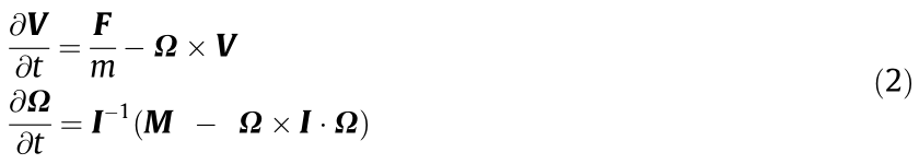
This section presents the mathematical equations of the nonlinear Boeing 747-100 aircraft model used in this study. The mathematical model is of a state-space model formulation derived from the general equation of motion of a rigid body. According to Newtonian mechanics, for a rigid body in motion, the rates of change of the linear and angular velocities are related to the total forces and moments acting on the body, as given by the following equation:

where F = and M = [L M N ]^T are the force and moment vectors along the x, y, and z axes in the body axis system, respectively; V = is the linear velocity vector, where u, v, and w are the velocity along the x, y, and z axes, respectively;  is the angular velocity vector, where p is roll rate, q is pitch rate, and r is yaw rate; m is the mass of the aircraft; t is time; and I is its constant inertia tensor (which are moments and products of inertia of the aircraft) [17]. Eq. (1) can be rewritten into a state-space formulation according to the following equation:

It is easily seen that Eq. (2) is of the standard state-space form and can be written in the general form as follows:

where are the states with the corresponding time derivatives denoted as ; R represents real number; K represents the total number of states; represents the time-variant inputs of dimension W; and is the disturbance vector (e.g., atmospheric disturbances) of dimension Z. It should be noted that Eq. (3) represents the nonlinear time-variant state equation in which the forces and moments exerted on aircraft are implicitly modeled.

It should also be noted that the nonlinear time-invariant equivalent of Eq. (3) generally suffices to model any realistic physical dynamical systems, including aircraft. Therefore, a nonlinear time-invariant model was assumed in this study. For example, although the moment of inertia may depend on many other factors such as the mass of aircraft, it is not dependent on time (i.e., age of aircraft). In the Boeing 747-100 aircraft model utilized in this study, the number of state variables is 13. In particular, the states include the standard 12-dimensional variable (which governs the body rates and accelerations) as well as an additional variable that has been called ‘‘pre-thrust” and represents the dynamics of the engine. The state equations are briefly described in Section 2.2.

《2.1. The Boeing 747-100 aircraft model》

2.1. The Boeing 747-100 aircraft model

The Boeing 747-100 is a four-fanjet jumbo transport aircraft that first came into operation in 1967. For taxiing, the Boeing 747-100 is equipped with a tiller and a rudder that facilitate directional control. Thrust is assumed to be generated using the two inner engines. The Boeing 747-100 is also equipped with inward and outward Krueger flaps and a movable stabilizer with four ailerons, but these are not included in the modeling as they are assumed to not be in use during taxiing. The datasets utilized for modeling the components of the Boeing 747-100 used in this study were obtained from Refs. [18,19].

The convention of the forces and moments acting in the body frame on the aircraft is shown in Fig. 1, while Fig. 2 shows the aircraft components that have been modeled in this study. It should be noted that the engine and fuel systems is modeled based on the International Civil Aviation Organization (ICAO) database.

《Fig. 1》

Fig. 1. The aircraft force and moment conventions.

《Fig. 2》

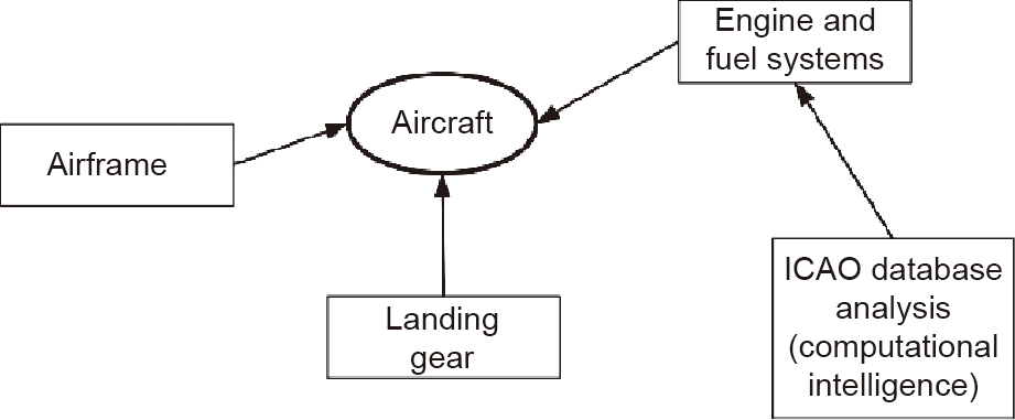
Fig. 2. The aircraft taxiing components and conventions. ICAO: International Civil Aviation Organization.

《2.2. State equations》

2.2. State equations

As mentioned above, the nonlinear state equations consist of 13 nonlinear functions. The states are subdivided into the following sub-states:

where x₁ ,x₂ , x₃ , x₄ , and x₅ represent the rotational velocity, trans-lational velocity, attitude, position, and pre-thrust sub-vectors, respectively. , , , , x_5 = pre-thrust: x₁ depends on the roll rate p, pitch rate q, and yaw rate r. x₂ is a function of velocity vector V, angle of attack α , and sideslip angle β. The attitude vector x₃ is a function of roll angle , pitch angle , and yaw angle . The position vector x₄ consists of the altitude h and the x and y positions. It is worth emphasizing that the rotational and translational velocities are defined within the body/wind axis of the aircraft, while the attitude and position are defined in the earth axis frame. The last variable represents the thrust, which is also given in the body axis of the air-craft. The vector function , which relates the vector states derivatives to the vector states and the inputs, is given by the following equation:

where represent the vector sub-functions that relate the rotational, translational, attitude, position, and prethrust vectors to the state variables, respectively. Each of these sub-functions (except for the pre-thrust variable) is derived in Ref. [20] but, for the sake of completeness, the sub-functions are summarized in Appendix A.

In the Boeing 747-100 aircraft model, the engine pressure ratio (EPR) or the pre-thrust determines the thrust produced by the aircraft. This is represented by a first-order dynamic system with a time constant of 5 s. It is necessary to convert this to the statespace form to make it compatible with other state equations and facilitate developing the model. Given the static EPR (steady state value), which is dependent on the throttle setting, the pre-thrust rate is given by the following equation:

where g is a function that relates the EPR to the throttle setting ðthrÞ and given states and represents the steady state EPR. Given the prethrust, the thrust generated by the engines can be calculated, as will be shown in Section 2.3. It should be noted that the state equations are applicable to any aircraft. However, the forces and moments data are typically peculiar to the aircraft. The derivations for the force and moment components as well as the dataset utilized are described in Section 2.3.

《2.3. Force and moment derivations》

2.3. Force and moment derivations

This section describes the forces and moment equations of the developed Boeing 747-100 aircraft model. The forces and moments equations include aerodynamic components, engine components, and undercarriage components whose data were obtained from Refs. [18,19].

2.3.1. Aerodynamic forces and moments

For taxiing, the aerodynamic forces and moments can be significant, especially at relatively higher speeds. The aerodynamic components of the forces and moments are all calculated in the wind axis and are then transformed into the body axis. The aerodynamic datasets are obtained in the form of unitless dimensional coefficients C_*. The subscript * is one of six subscripts that specify one of the six aerodynamic components, as shown in the Appendix A.

2.3.2. Engine forces and moments

The developed Boeing 747-100 aircraft model is equipped with four Pratt and Whitney JT9D-3 engines with a take-off thrust of 43 500 lbf (193 500 N). Only two engines have been assumed to be running throughout the simulations. It should be noted that the reverse thrust has not been utilized in modeling the aircraft engines, as it is not typically utilized during taxiing (it is only utilized from touchdown to about 100 knots (51 m·s^-1 ). A series of steps are necessary to calculate the final thrust generated by the engine, as follows:

(1) Obtain the throttle lever angle, and then use this angle to calculate the engine power lever angle (PLA). Note that in the Boeing 747-100 aircraft model developed here, this step has been somewhat modified so that the input to the system is a throttle setting normalized between 0 and 1. In particular, this means that the PLA of between 60° and 130° is transformed to be between 0 and 1 throttle in the developed Boeing 747-100 aircraft model. The normalization is performed using the following formula:

(2) Given the engine PLA (or thr normalized to between 0 and 1, as performed in the developed model), the static EPR is determined. The polynomial model relating thr to EPR is given by the following equation:

where k₀, k₁, k₂, and k₃ are the polynomial coefficients and are given in Table 1.

《Table 1》

Table 1 Coefficients of the polynomial function utilized for calculating the EPR.

(3) As already stated, the engine includes a transient, which is represented by a first-order dynamic system with a 5 s time constant. The static EPR calculated in the last step represents the reference level/steady state of the EPR. It is worth emphasizing that the transients have been represented in a state-space format, hence the need to add an additional state pre-thrust, as stated earlier. In essence, the pre-thrust variable represents the dynamic EPR.

(4) The National Aeronautices and Space Administration (NASA) reports in Refs. [18,19,21] provide plots for adding incremental EPR to the dynamic EPR as the Mach number of the aircraft increases. However, this has not been included in the simulation, as our taxiing speeds are typically less than 40 knots (21 m·s^-1 ), which would result in negligible incremental EPR due to the speed increase.

(5) When EPR is known (which is of course dynamic in nature), the final step involves calculating the net thrust per engine thrust. The net thrust is calculated as a function of the engine EPR as well as the ambient conditions. The equation for deriving the net thrust is given as follows:

where slope = 90° and intercept = -90° .

As calculations were performed using the international system of unit (SI) units in the developed model, thrust in the avoirdupois pound (lb) was converted into newtons by multiplying by the factor of 4.44822. It is worth emphasizing that the thrust derived in the preceding steps is for one engine only. In summary, the process of calculating the thrust developed per engine is shown in Fig. 3.

《Fig. 3》

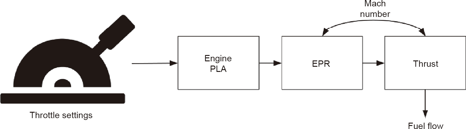
Fig. 3. Steps for calculating the net thrust.

Idle thrust: It is very important to note that at a throttle setting of zero, the EPR has an approximate value of 1.02, which makes the engine produce positive net thrust. It is also worth noting that the engines generate a moment about the center of gravity of the aircraft. While the net moment due to engine thrust is zero during the two-engine taxiing mode (in which inner engines are used and outer engines are switched off), for the single-engine taxiing mode, a moment will be produced that will make the aircraft yaw. This moment is easily calculated as the product of the force and the distance of the engine from the aircraft’s center of gravity. This distance is shown in Refs. [18,19] as being equal to 39.167 ft (11.938 m).

Fuel flow and emissions: Since one of the goals of this study is to find more efficient methodologies for aircraft taxiing, an accurate measure of engine fuel consumption and emissions is crucial. Consequently, an engine fuel consumption model based on the ICAO database of fuel and emissions [22] was developed. The ICAO database has been used extensively in the literature for studying the fuel consumption and emissions of engines at various thrust settings [15]. The database provides a comprehensive list of approximately 500 engines manufactured after 1980 as well as their fuel consumption and emissions at four distinct thrust settings. The distribution of the rated thrust of all the engines present in the database is shown in Fig. 4.

《Fig. 4》

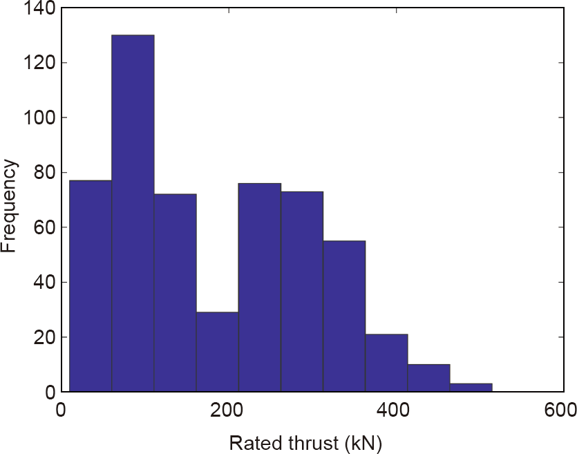
Fig. 4. Distribution of the rated thrust of the engines contained in the ICAO database.

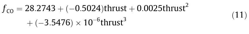
In addition to the emissions and fuel statistics shown in Ref. [22], the ICAO database includes other important information relating to the engine, such as out-of-production status, type of fuel, engine manufacturer, and whether or not the engine is out of service. The JT9D-3 engine was not present in the database list, which may be due to the fact that this engine was manufactured before 1980. To facilitate the calculations of fuel burn and emissions for the JT9D3 engine, a comprehensive statistical analysis of the database was undertaken. A fuzzy logic model has previously been utilized to analyze such data [23–25]. This analysis found that the rated thrust and out-of-production status of the engine were significant for predicting the fuel flow. Therefore, these two variables have been used for predicting the fuel flow of an arbitrary engine whose rated thrust and out-of-production status are known, as in the case of the JTD9-3 engine. The fuel flows at different values of thrust (four per engine) were arranged into a vector along with the engine out-ofproduction status. A polynomial was then utilized to identify a function that can be used for fuel flow and emission predictions. The data was divided into training and testing datasets (60% and 40%, respectively). The results of the polynomial regression are shown in Figs. 5(a) and (b). The rated thrust of the JT9D-3 engine is approximately 193.5 kN and the engine is currently out of production. These two variables were inputs into the polynomial regression model to predict the fuel flow and emissions. The results of such predictions are shown in Figs. 6(a) and (b). The fuel flow rate in Fig. 6(a) is calculated using a polynomial equation with the coefficients shown in Eq. (10). The carbon monoxide (CO) emission index in Fig. 6(b) is calculated in Eq. (11).

《Fig. 5》

Fig. 5. Result from predicting fuel flow given the rated thrust and the out-of-production status. (a) Training data results; (b) testing data results. RMS: root mean square.

《Fig. 6》

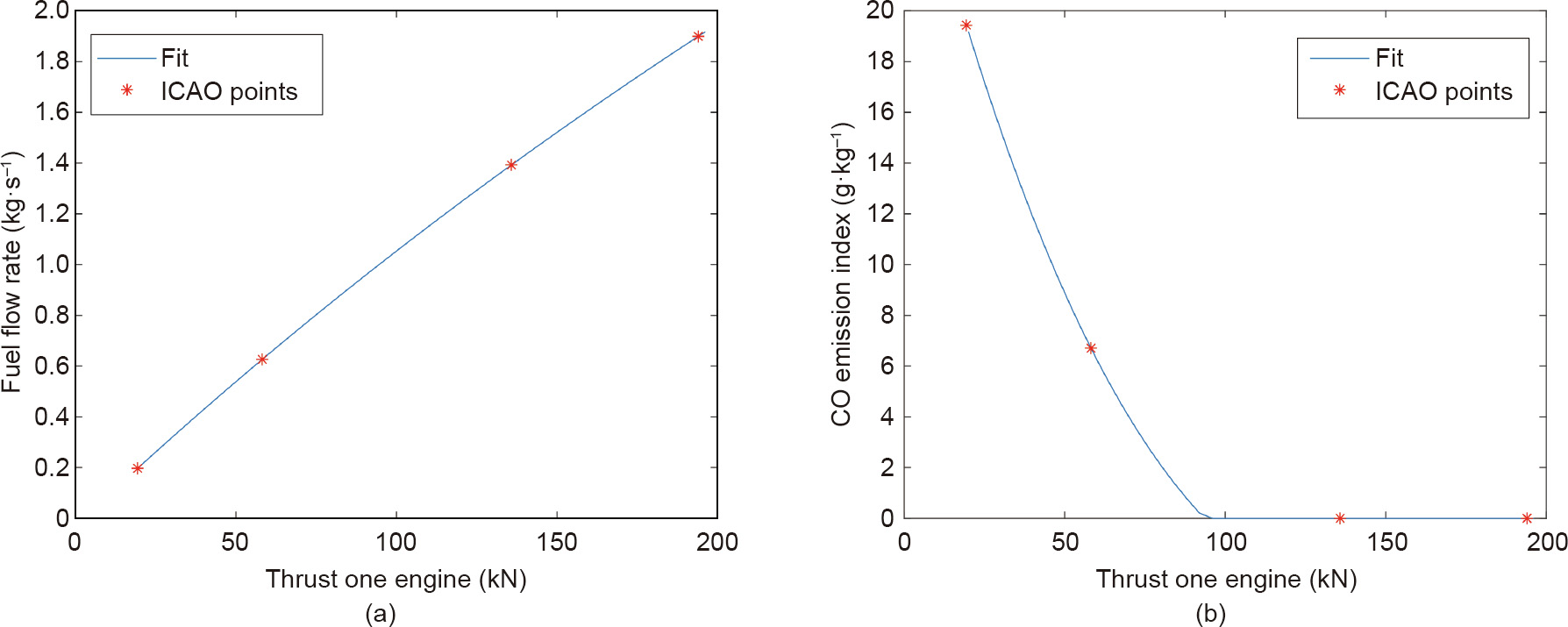
Fig. 6. Prediction for the JT9D-3 engine utilized in the Boeing 747-100 aircraft model. (a) Fuel flow; (b) carbon monoxide (CO) emission.

2.3.3. Undercarriage forces and moments

The data and the equations for calculating the forces and moments due to the undercarriage are given in Refs. [18,19]. The aircraft gears have been reconfigured into a tricycle model. In the tricycle model, the aircraft is assumed to have three gears and each gear is modeled as a nonlinear oleo-strut. There are two main gears (left and right) and one nose gear. The nose wheel is utilized for steering, but braking is only applied through the two main gears.

As the aircraft moves on the ground, the complex interaction between the ground, tires, and oleo-strut create forces and moments that affect the aircraft motion. The forces and moments due to the undercarriage are each calculated in the local axis of the gear and are each transformed into the body axis. As always, these forces and moments are dependent on the aircraft states. The steps by which these body forces and moments due to the undercarriage are calculated are as follows:

• Calculate the oleo-strut compression and rates: For each gear (nose gear, left main gear, and right main gear), the derivation of the compression and compression rates is shown in Fig. 7.

• Calculate vertical force: Once the oleo-strut compression and rates are determined, the three components of the forces (each in the local frame of the gears) are calculated. The first component involves calculating the vertical force F_z. The vertical force carries the weight of the aircraft and provides comfort for the passengers during taxiing. Calculating the vertical force in each gear involves determining two forces per gear (the damping force and the spring force) because the gear is represented by a nonlinear mass–damper–spring system. The spring force can be obtained from Refs. [18,19]. As in the case of the engine data used for calculating the static EPR, a polynomial fit was performed on the undercarriage data (for both the spring force and the damping constants for the main and nose gears).

• Calculate the side force: The aircraft taxiing movement requires a series of maneuvers that include turning. The turning motion is a consequence of the side forces acting from different components of the aircraft. Calculating the landing gear side force involves a series of steps. The first step involves determining the tire deflection variable based on the vertical force acting on the tire. This vertical force acting on the tire will be dependent on the attitude of the aircraft. The next step involves calculating the total side force. The total side force is the product of the angle between the tire and the direction of motion and the tire deflection constant. The total side force is limited to 60% of the total vertical force acting on the tires.

《Fig. 7》

Fig. 7. Derivation of the oleo compression and compression rates. and denote the oleo compression and oleo compression rates, respectively, at the ith gear for i = 1, 2, 3 (tricycle model assumed). Given and , this block diagram provides the necessary steps for deriving the vertical force. The vertical force acts upward from the tires toward the body of the plane along the struts. and are the body pitch and bank angles, respectively. x_i, y_i, and z_i are the distances of the ith gear to the center of gravity in body axes. The dots on and represent the derivative of these variables.

• Calculate the drag force: The drag force produces the braking forces, which are applied through the main gears and are used to stop or decelerate the aircraft during taxiing. At a particular gear, the drag force is dependent on a combination of braking and frictional forces. The braking is dependent on a constant K_B = 0.263, the aircraft mass, and the braking pedal deflection. The maximum amount of braking force is dependent on the aircraft mass, the rolling friction (μ_B = 0.4 for a dry taxiway), and a maximum braking constant (K_BM = 0.834 + 4.167 ×μ_B). The frictional force consists of two components (break-out force (bof) and a constant rolling friction term). The bof is dependent on the ground speed (V_G) of the aircraft and is determined as follows:

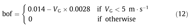
It is worth noting that the deflection of the braking pedal has been normalized to between 0 and 1.

• Transform the forces into the body axes: The forces derived above in each of the gears are then transformed into the body axis so that they can be included with the relevant body forces and moments. It was shown in Ref. [19] that the transformation equation is given by the following equation and is only valid for small angles:

where and are the body pitch and bank angles, respectively; and the indices 1, 2, and 3 specify the tire index. ,  , and are the tire drag force, vertical oleo strut force, and tire side force for the ith tire (note that ith tire is directly linked to the ith gear; therefore, we use the same subscript for clarity), respectively. is the nose wheel steering angle. The total undercarriage force is obtained by summing across the three gears, as follows:

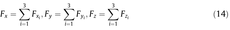
The moment equations are as follows:

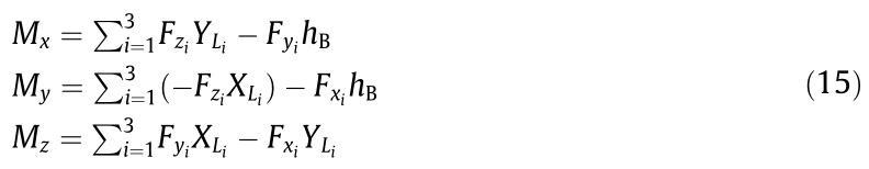
where X_L and Y_L are the distances from the center of gravity to the end of the fully extended landing gear. h_B = 17 + and is the vertical distance from the center of gravity of aircraft to the normal force, side force, and drag force created by the tires in contact with the runway. is oleo compression at the ith gear for i =1, 2, 3 (tricycle model assumed).

2.3.4. Gravity model

It is worth noting that there are two approaches by which the forces due to gravity can be incorporated into the aircraft model. The first approach involves implicitly including it in the translational acceleration function discussed earlier (Eq. (5)). The second involves explicitly stating the gravitational forces and then including them in the total forces and moments acting in the body frame of aircraft. The latter approach was used in modeling this aircraft. The gravity forces were assumed to act directly at the aircraft’s center of gravity, which indicates that there are no generated moments. The forces in the x (F_gx), y (F_gy), and z (F_gz), coordinates of the body frame are given by the following equation:

where GSA is the ground slope angle. An important consideration involves the way in which the ground slope of the taxiway has been included in the gravity model. If an aircraft is traveling downhill (a positive slope angle), then gas will cause a positive force along the x axis of the aircraft. It should be noted that the banking slope has been neglected.

《3. Aircraft navigation optimization》

3. Aircraft navigation optimization

The navigation system (Fig. 8) consists of several blocks that allow aircraft to move on the ground in an optimal manner. At a particular airport, the scheduler will typically provide a list of waypoints as well as time deadlines to meet each waypoint. These waypoints are typically determined by an optimal scheduling algorithm (e.g., the k-quickest path problem with time windows (k-QPPTW) algorithm [5] or the airport multi-objective A* (AMOA*) algorithm [26], and the aircraft is required to follow this schedule in an optimal manner. The navigation system consists of an outer loop controller (denoted by the speed and heading algorithm), which determines the references. In contrast to existing openloop approaches [27–29], these reference points are calculated online based on the distance to the next waypoint and the time deadlines. The inner loop control system moves the control inputs so that the aircraft follow the reference points. When automation is not present, the inner loop system controller is usually the pilot. The inner loop controller can, however, serve as a guide to the pilot on how best to move the controller inputs so that taxiing between waypoints is optimal (i.e., uses the minimum amount of fuel). Therefore, the main goal of this part is to develop an optimal controller so as to move aircraft through the taxiways while meeting the schedule, whether through full automation or acting as a decision support. The approach utilized here is based on tuning the parameters of the PID controller, which minimizes some set objectives such as the fuel consumed when following the schedule.

《Fig. 8》

Fig. 8. Block diagram of the navigation system.

《3.1. Outer loop control system》

3.1. Outer loop control system

The outer loop control determines the heading and speed when following a specified schedule. In this study, the outer loop control system is not optimized. The procedure by which the reference heading and speed are determined is given by the following example.

Example 1: Suppose the scheduler provides the following information to the outer loop controller: ‘‘Move aircraft along a straight line of distance 500 m in 50 s.” Then, the outer loop control system would generate the speed and heading references using the following steps:

(1) Determine the type of segment. The first step is to determine whether the movement to the specified waypoint involves passing through a turning or whether it is a straight line segment. The distance of the straight line segment is calculated in Step (2).

(2) Calculate the distance (D) to the next waypoint.

where are the coordinates of the waypoint and are the coordinates of the current aircraft position.

(3) Calculate the predicted distance, assuming the aircraft continue to move at the current speed. The predicted distance (D_pred) is given as follows:

where t_r is the time remaining to get to the waypoint and S_c is the current speed. The predicted distance is subtracted from the distance to the next waypoint to create the distance error variable (E).

(4) Calculate the reference using the following equation:

where S_ref is the reference to the inner controller, and is a constant that determines the rate of change of the reference speed. can also be optimized, but when it is not optimized, a value of = 10 was found, by trial and error, to work well.

(5) In some cases, a speed constraint is specified at the end (e.g., when moving from a straight segment into a turning segment, a fixed speed is to be used at that the turning segment). In such a case, the following algorithm is included to calculate the reference speed:

(i) Based on the current speed (S_c) and noting the maximum deceleration (1 m·s^-2) and maximum acceleration (also 1 m·s^-2), calculate the time (td) that would take based on the current speed for the aircraft to meet the required speed at the end. This time can be found by using the following equation: t_d = /1, where is the absolute difference between S_c and the specified speed at the waypoint (S_f).

(ii) Given t_d and assuming a constant rate of acceleration or deceleration, calculate the distance (D_d) required for such an acceleration/deceleration to meet the speed constraint at the waypoint. This can be calculated as follows:

(iii) Calculate a buffer distance (D_b) that determines the total distance traveled in trying to meet the speed constraint at the way point. This is calculated as follows:

The above equation determines the distance required to accelerate or decelerate to meet the required speed constraint at the waypoint.

(iv) If the remaining time deadline required to meet the waypoint is greater than t_d, then follow the normal control routine (as defined in steps (i)–(iii)) making sure to use D - D_b in place of D and t_r - t_d in place of t_r.

(v) If the remaining time deadline is, however, less than or equal to t_d, then set S_ref = S_f .

The proposed navigation algorithm described above has been tested using several scenarios that involve moving to/from the origin to the point (500 m, 0 m) in 50 s with an initial speed of 5 m·s^-1 and a final speed of 5 m·s^-1 . The result of testing the algorithm on the scenarios above is shown in Fig. 9.

《Fig. 9》

Fig. 9. (a) Reference and actual speeds of aircraft in a scenario where the final speed is specified (5 m·s^-1 ); (b) distance covered with time.

Indeed, it can be seen that the navigation system is able to reach the specified waypoint by the required time deadline. For turning segments, the above navigation algorithm is used but the distance is calculated in a different manner. To be specific, a constant turning rate is assumed (four degree per second), which is then utilized to calculate the time required to complete the turn and the time at which turning should commence.

《3.2. Inner loop control system》

3.2. Inner loop control system

Thus far, the discussion has only been concerned with how to determine the references (i.e., heading and speed). The inner control loop is responsible for manipulating the aircraft inputs (rudder, throttle, and braking) so that the aircraft follows the reference. The inner loop control consists of three sets of PID controllers with each PID controller respectively manipulating the throttle, brakes, and rudder. For braking, only the proportional controller is utilized. To avoid a scenario in which the brakes and throttle are used simultaneously, a function is included in the control block so that the brakes are used only when the aircraft speed is greater than the reference speed, while the throttle is used when the current speed is less than the reference speed. The configuration for the PID control system is shown in Fig. 10.

《Fig. 10》

Fig. 10. Configuration of the PID control system utilized in the inner control loop. P: proportional; PI: proportional–integral.

The PID parameters are optimally tuned for the scenarios of a taxiing aircraft at a given airport. Example 1 discussed earlier is a typical scenario. The optimization is performed using the genetic algorithms (GAs) in MATLAB (MathWorks, USA). The performance criteria are based on the fuel consumed to perform the task specified by the scenario. In summary, the objective function utilized for the optimization algorithm is given by the following equation:

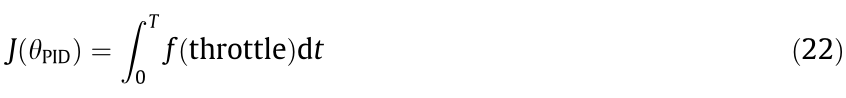
where J is the objective and represents the PID gains. T represents the time required to finish the schedule as determined by the scheduler, and (throttle) is the fuel consumption model elicited based on Fig. 5. As can be seen in Eq. (22), the throttle is dependent on the PID gains. It should be noted that the GA utilized in this study uses the value encoding methodology with a population size set to 1000. On average, the algorithms approximately converged at the 900 000th generation. One weakness of the above method is that the PID gains may not be optimal for another scenario. To find the optimal gains for a new scenario, the optimization algorithm needs to be run anew, which can incur significant computational costs when there is a large number of scenarios. Using the Manchester Airport (UK) as a case study, the scheduler included approximately 90 000 scenarios (Fig. 11(a)). Evidently, it is not feasible to obtain 90 000 sets of optimal PID gains. To solve this problem, it is proposed to carry out a cluster analysis on the scenario lists. The center of the cluster is assumed to be representative of the cluster members. The optimization is performed only on those scenarios that represent the cluster centers, and the PID gains of the particular center are utilized across the whole cluster members. The result of the cluster analysis for the case of the Manchester Airport is shown in Fig. 11(b).

《Fig. 11》

Fig. 11. (a) Scatter plot of the scenarios; (b) cluster analysis of the scenarios in which six clusters are presented with red dots indicating the centers of each cluster.

Table 2 includes details of the result of utilizing the clustered PID control approach as compared with two other methodologies on ten randomly chosen scenarios. The first relates to choosing a controller randomly from the six controllers, and the second involves choosing a fixed controller for all the scenarios chosen.

《Table 2》

Table 2 Comparison of the results of three control strategies.

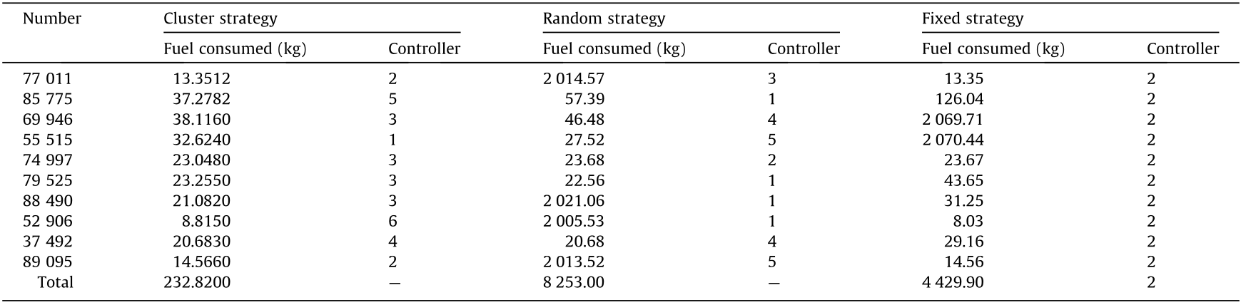
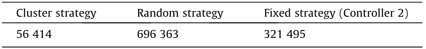
As can be seen from Table 2, using a clustering strategy results in a significantly better performance than using just one controller for all scenarios. It should be noted that a penalty term (2000 kg of fuel consumed) has been included for scenarios where the control strategy violates the scheduler or aircraft constraints. The total fuel consumed from the three different control strategies for the 1000 randomly chosen scenarios is shown in Table 3. It can be seen that, on average, the clustering-based approach consistently provides better performances than a strategy using a fixed controller.

《Table 3》

Table 3 Total fuel consumed for 1000 randomly chosen scenarios. Controller 2 provided the best performance out of all the other controllers for the fixed strategy method.

《4. Results》

4. Results

The proposed approach was tested on two scenarios, as discussed in the following subsections.

《4.1. Taxiing run along a rectangular path》

4.1. Taxiing run along a rectangular path

The first scenario relates to taxiing along a rectangular layout, which is shown in Fig. 12.

《Fig. 12》

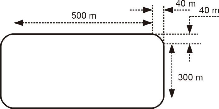
Fig. 12. Rectangular layout used for testing.

The schedule for the aircraft to follow was chosen so as to take into account the constraints of the aircraft during taxiing, such as maximum acceleration, deceleration, and the limits of the turning rates. The schedule includes two categories of taxiing runs. The first taxiing run involves taxiing along the rectangular path with the assumption that there is no ground slope. The second involves taxiing along the rectangular path with the assumption of a ground slope of 2°. Incorporating the slope is important because aircraft may taxi across different taxiways that include significant ground slopes. The starting point of aircraft is taken to be the left end of the straight portion of the base of this rectangle. From this point, the layout is divided into eight different segments. The loci of the geodetic positions attained are plotted for different segments of the path, as shown in Fig. 13. Time deadlines for the simulated segments are shown in Table 4.

《Table 4》

Table 4 Segment-wise time deadlines chosen for the simulation.

《Fig. 13》

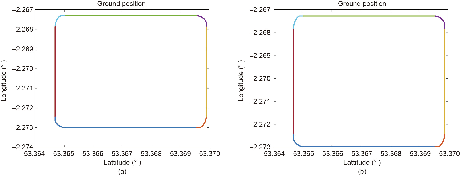
Fig. 13. Geodetic positions of the aircraft during the rectangular layout test compared with the actual path. (a) No slope taxiing; (b) taxiing at 2° slope angle.

The result of the taxiing run shown in Fig. 14 indicates that the aircraft is able to follow the specified route while keeping to the schedule.

《Fig. 14》

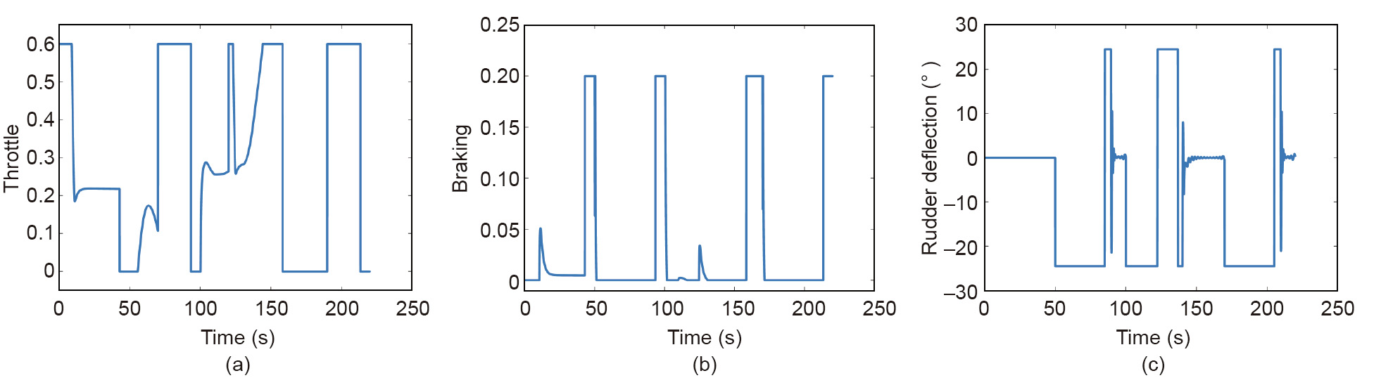
Fig. 14. Input profiles for taxiing through the rectangular segment with a slope of 0°. (a) Throttle; (b) braking; (c) rudder deflection.

《4.2. Taxiing run at Manchester International Airport》

4.2. Taxiing run at Manchester International Airport

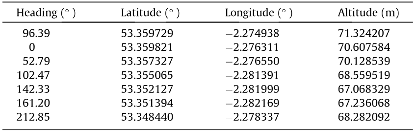
The proposed algorithm was tested on a real-life taxiing study that involved taxiing from the gate to the runway holding point (ready to take off) at the Manchester International Airport in the UK. The taxiway layout of the airport and the optimized route from the scheduler are shown in Fig. 15. The coordinates of the waypoints are shown in Table 5.

《Table 5》

Table 5 Geodetic coordinates of the waypoints as outputted from the scheduler algorithm.

《Fig. 15》

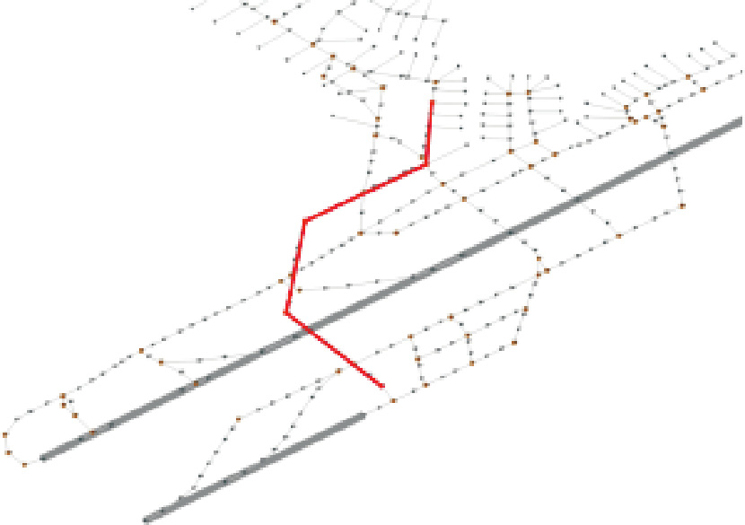
Fig. 15. Taxiway and runway layout of Manchester International Airport. The optimized taxi route is highlighted in red.

As can be seen in Fig. 16, when taxiing at the Manchester International Airport, the proposed approach results in fuel savings of about 11% compared with the conventional Ziegler–Nichols tuned PID approach.

《Fig. 16》

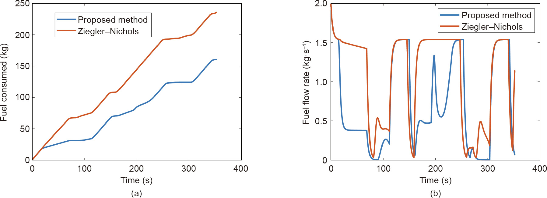
Fig. 16. Fuel consumed using the optimized PID gains for navigating the aircraft around the waypoints of the Manchester International Airport compared with the fuel consumed using a Ziegler–Nichols tuned PID. (a) Cumulative fuel consumed taxiing through Manchester Airport; (b) rate of fuel consumption for taxiing through Manchester International Airport.

《5. Conclusions》

5. Conclusions

This paper presented an approach for the optimal navigation of taxiing aircraft across a real airport. Although the algorithms were developed and tested based on a Boeing 747-100 aircraft model, the proposed approach is generic. The proposed approach involves optimizing the PID gains using a genetic algorithm so that taxiing is performed in an optimal manner. This method can be employed for a fully automated taxiing aircraft or can act as a decision support for the pilot through which he or she is advised on the optimal control inputs able to meet the time deadline of the scheduler while performing the maneuvers in an optimal manner. When tested on a real-life taxiing problem, the proposed approach was shown to save as much as 11% of fuel burn in comparison with popular heuristically tuned PID controllers. Indeed, the results presented in this paper represent an important leap in the quest to guide aircraft from gate to gate across the world. This approach not only opens the door for more efficiently running aircraft operations, but also helps to reduce aircraft fuel consumption, which is a significant contributor to greenhouse gas emissions. Future studies will attempt to quantify the effects of the many sources of uncertainties in aircraft ground movement, such as pilot behavior and different aircraft configurations.

《Acknowledgements》

Acknowledgements

This work was funded by the UK Engineering and Physical Sciences Research Council (EP/N029496/1, EP/N029496/2, EP/ N029356/1, EP/N029577/1, and EP/N029577/2).

《Compliance with ethics guidelines》

Compliance with ethics guidelines

Olusayo Obajemu, Mahdi Mahfouf, Lohithaksha M. Maiyar, Abrar Al-Hindi, Michal Weiszer, and Jun Chen declare that they have no conflict of interest or financial conflicts to disclose.

《Appendix A. Supplementary data》

Appendix A. Supplementary data

Supplementary data to this article can be found online at https://doi.org/10.1016/j.eng.2021.01.009.