

《1. Introduction》
1. Introduction
Oil sands ore contains bitumen, water, and minerals. Bitumen is a high-viscosity hydrocarbon mixture, which can be extracted by means of several chemical and physical processes. The product is further treated in upgrader units or refineries [1] to obtain more valuable byproducts (e.g., gasoline, jet fuel). Oil sands are mined from open pits and loaded into trucks to be moved into the crushers [2]. Following this, the mixture is treated with hot water for hydro-transportation to the extraction plant. Aeration and several chemicals are introduced to enhance this process. In the extraction plant, the mixture is settled down in a primary separation vessel (PSV). A water-based oil sands separation process is summarized in Fig. 1.
《Fig. 1》
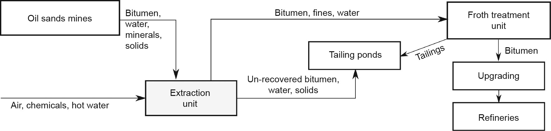
Fig. 1. A simplified illustration of the water-based oil sands separation process. The PSV is located in the extraction unit.
During the separation process inside the PSV, three layers are formed: froth, middlings, and tailings (Fig. 2). An interface (referred to as the froth–middlings interface (FMI) henceforth) is formed between the froth and middlings layer. Its level with reference to the PSV unit influences the quality of the extraction.
《Fig. 2》
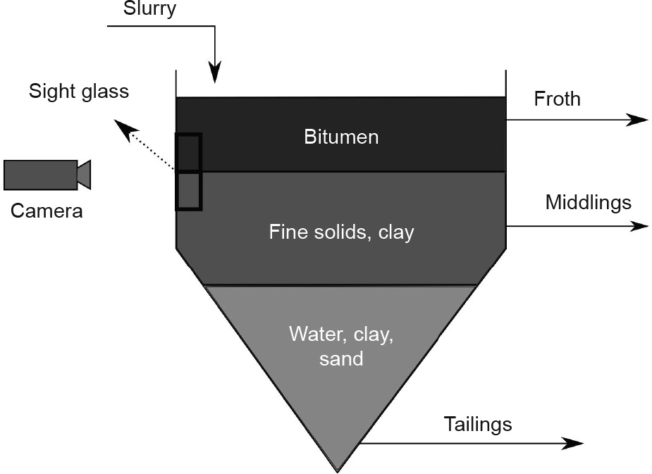
Fig. 2. A schematic of the PSV. During the separation process, three layers are formed. The camera is used to monitor the interface between the middlings and the froth layers in order to control the FMI level optimally.
To control the FMI level, it is crucial to have reliable sensors. Traditionally, differential pressure (DP) cells, capacitance probes, or nucleonic density profilers are used to monitor the FMI level. However, these are either inaccurate or reported to be unreliable [3]. Sight glasses are used to manually monitor the interface for any process abnormalities. To utilize this observation in closedloop control, Ref. [3] proposed using a camera as a sensor. This scheme utilizes an edge detection model with particle filtering on the images to obtain the FMI level; feedback control is then established using this model. More recently, Ref. [4] combined edge detection with dynamic frame differencing to detect the interface. This method directly uses the edge detection technique to detect the interface, along with a frame-comparison mechanism that estimates the quality of the measurement; it also detects faults. Ref. [5] used a mixture of Gaussian distributions to model the appearances of the froth, interface, and middlings, and predicted the interface using a spatiotemporal Markov random field. Despite addressing several challenges utilizing models based on the appearance or behavior of the interface, these techniques fail to address the sensitivities to uncertain environmental conditions, such as occlusion and excessive/non-Gaussian noise.
Supervised learning (SL) methods try to build a map from input (i.e., image, x) to output (i.e., label, y) data by minimizing a cost (or loss) function. Usually, the cost function is convex, and the optimal parameters are calculated by applying a stochastic gradient descent algorithm [6,7] to the cost function. Unsupervised learning (UL) methods, on the other hand, are used to find the hidden features in the unlabeled data (i.e., uses x only) [8]. The goal is usually to compress the data or to find similarities within the data. Nevertheless, UL techniques do not consider the impact of the input on the output, even if such a causal relationship exists. In computer vision, these methods are implemented using convolutional neural networks (CNNs). A CNN is a parametric function that applies convolutional operation on the inputs. It can extract abstract features by processing not just a pixel, but also its neighboring pixels. It is used for classification, regression, dimensionality reduction, and so forth [9–12]. Even though they have been used for decades [13–16], CNNs have only lately gained significant popularity in different domains [17–20]. This is due to the developments that have occurred in hardware technology [21] and data availability [22]. Parallel to the developments in computer vision, a recurrent neural network (RNN) is used for time-series prediction, where the previous output of the network is fed back into itself [23] in what can be considered a recursive matrix multiplication. However, vanilla RNN [24] suffers from diminishing or exploding gradients, because it repeatedly feeds the previous information back into itself, leading to uneven back-propagated data sharing in between hidden layers. Therefore, it tends to fail when the data sequence is arbitrarily long. To overcome this issue, more complex networks such as long short-term memory (LSTM) [25] and gated recurrent units [26] have been proposed. These networks facilitate data transfer in between hidden layers to make the learning more efficient. More recently, a variant of LSTM called convolutional LSTM (ConvLSTM) [27] was reported to improve LSTM performance by replacing matrix multiplications with convolutional operations. Unlike fully connected LSTM, ConvLSTM receives an image rather than onedimensional data; it utilizes spatial connections that are present within the input data and enhances estimation. Networks with many layers are considered to be deep structures [28]. Various deep architectures have been proposed [29–33] to enhance the prediction accuracy even further. However, these structures suffer from over-parameterization (i.e., the number of training data points is less than the number of parameters). Several regularization techniques (e.g., dropout, L2) [17] and transfer learning (also called fine-tuning (FT)) methods [34,35] try to find a work-around to improve the network’s performance. However, the transferred information (e.g., network parameters) may not be general enough for the target domain. This issue becomes significant, especially when the training data is insufficient or their statistics are significantly different than the data in the target domain. Moreover, efficient transfer learning for recurrent networks currently remains as an opportunity for further research.
Reinforcement learning (RL) [36] combines the advantages of both SL and UL techniques and formalizes the learning process as a Markov decision process (MDP). Inspired by animal psychology [37] and optimal control [38–43], this learning scheme involves an intelligent agent (i.e., the controller). Unlike SL or UL methods, RL does not rely on an offline or batch dataset, but generates its own data by interacting with the environment. It evaluates the impacts of its actions by considering immediate consequences and predicts the value via roll-out. Hence, it is more suitable for real or continuous processes involving decision-making for complex systems. However, in sampled data-based schemes, data distribution may be significantly different during training, which may cause high variance of estimations [36]. Actor–critic methods have been proposed [44–46] in order to combine the advantages of value estimation and the policy gradient. This approach segregates the agent into two parts: The actor decides which action to take, while the critic estimates the goodness of that action using an action-value [47] or state-value [48] function. These methods do not rely on any labels or system models. Therefore, exploration of the state or action space is an important factor that affects the agent’s performance. In system identification [49–51], this is known as the identification problem. Various methods have been developed to address the exploration issue [36,48,52–58]. As a subfield of machine learning [59–61], RL is used in—but not limited to—process control [2,42,61–68], the game industry [69–77], robotics, and autonomous vehicles [78–81].
FMI tracking can be formulated as an object-tracking problem, which can be solved in one or two steps using detection-free or detection-based tracking approaches, respectively. Previous works [82–84] have used RL for object detection or localization, for which it can be combined with a tracking algorithm. In the case of such a combination, the tracking algorithm also needs to be reliable and fast for real-time implementation. Several object-tracking algorithms have been proposed, including multiple object-tracking algorithms using RL [85–90]. The proposed schemes combine pretrained object detection with RL-based tracking or a supervised tracking solution. These simulations were carried out under ideal conditions [91,92]. The performance of object-detection-based methods often depends on the detection accuracy. Even if the agent learns to track based on a well-defined reward signal, the researcher should ensure that the sensory information is (or the features of the sensory information are) accurate. Model-based algorithms often assume that the object of interest has a rigid or a non-rigid shape [4] and that the noise or the motion has a particular pattern [3]. These assumptions may not hold when unexpected events occur. Therefore, a model-free approach may provide a more general solution.
Since a CNN may extract abstract features, it is important to analyze it after training. Common analysis techniques utilize the information of the activation functions, kernels, intermediate layers, saliency maps, and so forth [30,93–95]. In an RL context, a popular approach has been to reduce the dimensions of the observed features using t-distributed stochastic neighbor embedding (t-SNE) [96] to visualize the agent in different states [72,97,98]. This helps to cluster the behavior with respect to the different situations encountered by the agent. Another dimensionalityreduction technique—namely, uniform manifold approximation and projection (UMAP) [99]—projects the high-dimensional input (which may not be meaningful in the Euclidean space) into Riemannian space. In this way, the dimensionality of nonlinear features can be reduced.
Fig. 3 illustrates a general control hierarchy in the process industry. In a continuous process, each level in the hierarchy interacts with each other at different sampling frequencies. Interaction starts at the instrumentation level, which affects the upper levels significantly. Recently, Ref. [2] proposed a solution for the execution level. However, addressing other levels remains challenging.
《Fig. 3》

Fig. 3. A general control hierarchy in the process industry. RTO: real-time optimization; MPC: model predictive control; PID: proportional–integral–derivative controller.
Here, we propose a novel interface tracking scheme based on RL that is trained for a model-free sequential decision-making agent. This work:
• Provides a detailed review of actor–critic algorithms;
• Focuses on the instrumentation level to improve the overall performance of the hierarchy;
• Formulates interface tracking as a model-free sequential decision-making process;
• Combines CNN and LSTM to extract spatiotemporal features without any explicit models or unrealistic assumptions;
• Utilizes DP cell measurements in a reward function without any labels or human intervention;
• Trains the agent using temporal difference learning that allows the agent to learn continuously in a closed-loop control setting;
• Validates robustness amidst uncertainties in an open-loop setting;
• Analyzes the agent’s beliefs in a reduced feature space.
This paper is organized as follows: Section 2 provides a review on actor–critic algorithms and preliminary information, interface detection is formulated in Section 3, Section 4 presents the training and test results in detail, and conclusions and future work are drawn in Sections 5 and 6, respectively.
《2. Review of actor–critic reinforcement learning》
2. Review of actor–critic reinforcement learning
RL is a rigorous mathematical concept [36,39,42] in which an agent learns a behavior that maximizes an overall return in a dynamic environment. Similar to a human being, the agent learns how to make intelligent decisions by considering the future rewards. This implies contemplating temporal aspects of the observations, unlike simple classification or regression approaches. This ability allows RL to be used under uncertain conditions [40] with irregular sampling rates. Its versatile nature makes RL adaptive to different environmental conditions and allows it to be transferred from simulation environments to real processes [80].
《2.1. Markov decision processes》
2.1. Markov decision processes
An MDP formulates discrete sequential decision-making processes via a tuple, M, that consists of  , where
  are the state, action, and reward, respectively.
  represents the system dynamics, or state transition probabilities, which may be deterministic or stochastic. It satisfies the Markov property [100]—that is, the future state depends solely on the current state, and does not depend on the history prior to that. In this work, system dynamics are unknown to the agent in order to make this approach more general. The discount factor
  is a weight for future rewards in order to make their summation bounded. The stochastic policy,
  , is a mapping from the observed system states to the actions.
In an MDP, the agent observes a state  , where
  represents the distribution of the initial states. It then selects an action
  that carries the agent to a next state,
  , and yields a reward,
  . By utilizing the sequence
  , the agent learns a policy, π , that leads to maximizing the discounted return, G, as defined in Eq. (1) [36]:

where t and k represent discrete timestep. The state-value,  , and action-value,
  , functions are calculated using the Bellman equations (Eqs. (2) and (3)):
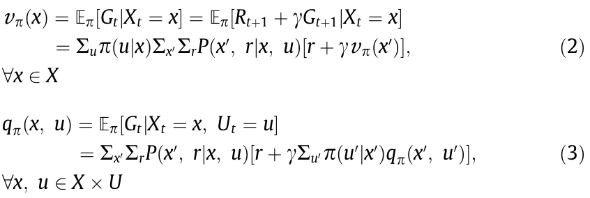
where  is the expectation of a random variable. After the value functions are estimated for each state, the optimal value (
  and
and  ) functions can be found using Eqs. (4) and (5):

Following that, the optimal policy, π *, can be found as follows:

For largescale problems, linear or nonlinear function approximation techniques can be used to find the approximated value functions,  or both, where
  represents the parameters of the approximated unctions. These structures are also called critics. This work focuses on the state-value estimation and simplifies its notation as V(∙).
《2.2. A review of actor–critic algorithms》
2.2. A review of actor–critic algorithms
Earlier approaches used value-based (critic-only) RL [71,101] to solve control problems. In these approaches, actions are derived directly from a value function, which has been reported to be divergent for largescale problems [45,102]. Policy-based (actoronly) methods [103–105] tackle this problem and can learn stochastic behaviors by generating a policy directly from a parameterized function. This function is then directly optimized by using a performance metric. However, variance of the estimation and the extended learning time make the policy gradient impractical. Similar to generative adversarial networks (GANs) [106], which utilize generative and discriminative networks, actor–critic algorithms self-supervise without any labels [44,45,107,108]. These techniques combine policy and value-based methods via an actor and a critic, respectively. This assisted estimation reduces the variance significantly and helps in learning the optimal policy [36,55]. The actor and the critic can be represented as two neural networks,  (where
  represents the parameters of the actor network) and
  (or
(or  ), respectively.
Although several model-based actor–critic schemes have been proposed [109,110], this paper focuses on the most commonly used model-free algorithms, as represented in Table 1. Some of these methods use entropy regularization, whereas the others take advantage of heuristic methods. A common example for these methods is the  -greedy approach, in which the agent takes a random action with a probability
  . Other exploration techniques include—but are not limited to—introducing additive noise to the action space, introducing noise to the parameter space, and utilizing an upper confidence bound. Interested readers can see Ref. [67] for more detail.
The actor–critic algorithms are summarized as follows.
《Table 1》
Table 1 A comparison of actor–critic algorithms based on the type of action spaces and the exploration method. The state space can be either discrete or continuous for all the algorithms.

DDPG: deep deterministic policy gradient; A2C: advantage actor–critic; A3C: asynchronous advantage actor–critic; ACER: actor–critic with experience replay; PPO: proximal policy optimization; ACKTR: actor–critic using Kronecker-factored trust region; SAC: soft actor–critic; TD3: twin delayed deep deterministic policy gradient.
2.2.1. Deep deterministic policy gradient
This algorithm has been proposed to generalize discrete, lowdimensional value-based approaches [71] to continuous action spaces. The deep deterministic policy gradient (DDPG) [47] utilizes an actor and a critic (Q) as well as a target critic (Q' ) network, which is a copy of the critic network. After observing a state, real-valued actions are sampled from the actor network and are mixed with a random process (e.g., the Ornstein–Uhlenbeck process) [111] to encourage exploration. The agent stores state, action, and reward samples in an experience replay buffer to break the correlation between consecutive samples in order to improve learning. It minimizes the mean square error of the loss function, L, to optimize its critic, as shown in Eq. (7).

The scheme utilizes a policy gradient to improve the actor network. Since the value function is learned for the target policy based on a different behavior policy, DDPG is an off-policy method.
2.2.2. Asynchronous advantage actor–critic
Instead of storing the experience in a replay buffer that requires memory, the asynchronous advantage actor–critic (A2C/A3C) scheme [48] involves local workers that interact with their environments and update a global network asynchronously, which inherently increases exploration. Instead of minimizing the error based on the Q function, this scheme minimizes the mean square error of the advantage function (A or δ) for the critic update, as shown in Eq. (8).

In this scheme, the global critic is updated by using Eq. (9), and the entropy of the policy is used as a regularizer in the actor loss function to increase exploration, as shown in Eq. (10):
where initially  . A left arrow (
  ) represents the update operation;
  and
and  are the learning rates for the critic and actor, respectively;
  is the derivative with respect to its subscript; and β is a fixed entropy term that is used to encourage exploration. Subscripts L and G stand for the local and global networks, respectively. Multiple workers (A3C) can be used in an offline manner, and the scheme can be reduced to a single worker (A2C) to be implemented online. Even though the workers are independent, they predict the value function based on the behavior policy of the global network, which makes A3C an on-policy method. This work utilizes an A3C algorithm to track the interface.
2.2.3. Actor–critic with experience replay
The actor–critic with experience replay (ACER) method [112] addresses the sample inefficiency of the A3C by utilizing a Retrace algorithm [113], which estimates Eq. (11):

where the truncated importance weight,  ,
,  , and c is a clipping constant. μ1 and μ2 are the target and the behavior policies, respectively. Moreover, this scheme utilizes stochastic dueling networks (to estimate both V and Q in a consistent way) and a trust region policy optimization (TRPO) method that is more efficient than the previous method [114]. Because of its Retrace algorithm, ACER is an off-policy method.
2.2.4. Proximal policy optimization
The proximal policy optimization (PPO) method [115] improves TRPO [114] by clipping the surrogate objective function, as shown in Eq. (12):

where  represents the policy parameters (i.e.,
  represents the old policy parameters),
  , and
, and  is the clipping constant. A is the advantage estimate that represents how beneficial the agent’s actions are, as shown in Eq. (8).
2.2.5. Actor–critic using Kronecker-factored trust region
Instead of a gradient descent [6] algorithm to optimize the actor and critic networks, the actor–critic using Kronecker-factored trust region (ACKTR) [116] utilizes second-order optimization, which provides more information. It overcomes the computational complexity by using Kronecker-factored approximation [117,118] to approximate the inverse of the Fisher information matrix (FIM), which otherwise scales exponentially with respect to the parameters of the approximation. Moreover, it keeps track of the Fisher statistics, which yields better curvature estimates.
2.2.6. Soft actor–critic
Unlike methods that use the entropy of the policy as a loss regularizer [48,114,115,119], the soft actor–critic (SAC) method [55,120] augments the reward function with the entropy term (as shown in Eq. (13)) to encourage exploration. This approach has also been reported [120] to improve the robustness of the policy against model errors.

where represents the parameters of the policy, α is a user-defined (fixed or time-varying) weight to adjust the contribution of the entropy, and  . This scheme relies on both the Q and V functions to utilize the soft-policy iteration. Similar to DDPG and ACER, SAC stores the transitions in a replay buffer to address sample efficiency. Besides enhancing the exploration, entropy maximization compensates for stability loss, which is introduced by the off-policy approach.
2.2.7. Twin delayed deep deterministic policy gradient
The twin delayed deep deterministic policy gradient (TD3) [121] addresses error propagation (which is a non-trivial challenge in statistics and control) [122] due to function approximation and bootstrapping (i.e., instead of an exact value, using an estimated value in the update step). To achieve it, the scheme predicts two separate action-values and prefers the pessimistic value; hence, it avoids suboptimal policies. TD3 utilizes target networks, delays the update to the policy function, and uses an average target value estimate by sampling N transitions from a replay buffer to reduce variance during learning. The scheme introduces exploration by adding Gaussian noise to the sampled actions and performs policy updates using the deterministic policy gradient [104].
Although the abovementioned algorithms provide general solutions to control problems, they may remain inadequate for more complex or specific tasks. Many other algorithms have been proposed to address these shortcomings. For example, Ref. [123] extended the discrete actor–critic method proposed by Ref. [44] to continuous time and space problems via the Hamiltonian– Jacobi–Bellman (HJB) equation [39,124]. This proposed algorithm was then tested in an action-constrained pendulum and a cartpole swing up problem. Ref. [125] employed an actor–critic algorithm on a constrained MDP together with a detailed convergence analysis. Ref. [46] showcased four incremental actor–critic algorithms based on regular and natural gradient estimates. Ref. [126] introduced a natural actor–critic (NAC) and demonstrated its performance on the cart-pole problem as well as on a baseball swing task. Ref. [127] presented a continuous time actor–critic via converse HJB and tested the convergence in two nonlinear simulation environments. Ref. [128] proposed an online actor–critic algorithm for an infinite horizon, continuous time problems with a rigorous convergence analysis, and linear and nonlinear simulation examples. Ref. [129] proposed an incremental, online, and off-policy actor–critic algorithm. The proposal analyzed the convergence qualitatively and supported it with empirical results. Moreover, the temporal difference (TD) methods were compared with gradient-TD methods that minimize the projected Bellman error [36]. Ref. [130] proposed an actor–critic identifier that could provably approximate the HJB equation without a knowledge of the system dynamics. After the learning was complete, the scheme showed process stability. However, knowledge of the input gain matrix was required. Ref. [131] used a nominal controller as a supervisor to guide the actor and to yield a safer control in a simulated cruise-control system. Ref. [132] proposed learning the solution of an HJB equation for a partially unknown inputconstrained system without the persistent excitation conditions while preserving the stability. By considering Lyapunov theory, Ref. [133] designed a fault-tolerant actor–critic algorithm and tested its stability on the Van der Pol system. Ref. [134] formulated an input-constrained nonlinear tracking problem by using the HJB equation and a quadratic cost function to define the value function. The scheme obtained an approximate value function with an actor–critic algorithm. Ref. [135] combined classification and time-series prediction techniques to solve an optimal control problem and showcased the proposed algorithm on a simulated continuous stirred-tank reactor (CSTR) and a simulated nonlinear oscillator. The mean actor–critic algorithm [136] was proposed to estimate the policy gradient by using a smooth Q function, which was averaged over the actions to reduce variance; the results were demonstrated on Atari games. Ref. [137] utilized an event-triggered actor–critic scheme to control a heating, ventilation, and air conditioning (HVAC) system. In addition to these, there are more recent studies on different actor–critic algorithms and their applications, as reported in Refs. [2,62,67,138–145].
Several methods have been proposed to improve value estimation in RL [146–148], which can be used in actor–critic algorithms. Moreover, different techniques [112,149] have been reported to improve the sample efficiency (i.e., to reduce the amount of data needed to learn the optimal policy). Unlike techniques that made use of experience replay [70] or supervised data [150], ‘‘parallel learning” makes use of multiple randomly initialized workers (local networks) that interact with different instances of the environment independently to reduce the variance in the policy during learning. These workers have the same infrastructure as a global network and, after collecting k-samples, are used to update parameters of the global network. This reduces the amount of memory used and improves exploration, because the workers have independent trajectories. Task distribution can be performed via multiple machines [151] or multiple central processing unit (CPU) threads of a single computer [48].
The optimal policy and the optimal critic are different in each process, and they are often unknown a priori. Monte Carlo-type methods calculate empirical return (given in Eq. (1)) at the end of the process (or an episode), which may be lengthy and noisy. Similar to Pavlovian conditioning [152] in psychology, TD learning predicts the value of the current state. Unlike Monte Carlo methods, it makes the predictions for a small horizon, as low as one step. This converts the infinite horizon problem into a finite horizon prediction problem. Instead of calculating the expectation of returns (as in Eq. (2)), the critic network can be updated using k-step ahead estimation of the TD error, δ, as shown in Eq. (14). This is called policy evaluation.
where δ is the TD error for state x at a discrete sampling instant, t, given the critic parameters of the local network  , and k represents the horizon length. If k approaches infinity, the summation terms converge to the empirical return given in Eq. (1). A baseline,
  , is used to reduce the variance compared with the policy gradient algorithm [36].
At the end of k steps, the parameters of the global network (i.e.,  and
and  ) are updated using Eqs. (9) and (10).
《3. Formulating the interface tracking as a sequential decisionmaking process》
3. Formulating the interface tracking as a sequential decisionmaking process
《3.1. Interface tracking》
3.1. Interface tracking
A model is a mathematical means of describing the process dynamics that can occur either in a physical/chemical/biological system [153] or in a video [154]. The models derived for images often suffer from inaccuracies when there is an unexpected event (e.g., occlusion). To overcome this, either the information from the last valid observation is used in the next observation [4] or the images are reconstructed [154]. Although these solutions may substitute actual measurements for a short period of time, prolonged exposure can deteriorate closed-loop stability. As a consequence, if the FMI’s level is too low, the bitumen from the froth layer drains into the tailings. This lowers the product quality and creates environmental footprints. In contrast, if its level is closer to the extraction point, the solid particles in the froth being extracted complicate downstream operations [3]. Since deviations in the FMI level affect the downstream processes, it is important to regulate the FMI at an optimum point.
RL can address inaccuracies during occlusion and excessive noise. This can be done by combining DP cell measurement or measurement from any other reliable instrument with the current FMI prediction by the agent to provide an accurate cost in the reward function, without external labels such as bounding boxes, during the training phase. Removing the dependence upon such labels minimizes human error. To achieve this, an agent can move a cropping box on the vertical axis over the PSV’s sight glass and compare its center with the DP cell measurement. Based on this deviation, the agent can move the box to an optimal position, where the center of the box matches to that of the FMI. This deviationminimizing feedback mechanism is inspired from control theory, and it can enhance an image-based estimation using the measurement obtained from the real process.
Consider a grayscale image, I, sampled from a video stream as  with an arbitrary width, W, and height, H, which captures the entire PSV. Consider a rectangular cropping box,
  , that has an arbitrary width, M, and height, N, where
  and
and  is the center of the rectangle. An example image and a cropping box are shown in Fig. 4(a). This rectangle crops I at into a size of N ×M. For the sake of completeness, H>N and W=M. Consider an interface measurement obtained from a DP cell at time t as z. Note that the DP cell is used only in offline training of the RL agent and can be replaced by other interface measurement sensors, which is considered to be accurate in the offline laboratory environments.
《Fig. 4》

Fig. 4. A frame (I) obtained using a camera. (a) Sizes of the image (H × W) and the cropping box (N × W); (b) sizes of the cropping boxes (N × M) and the initial cropping box positions; (c) an example occlusion with its ratio, ρ.
The components of the MDP for this problem can then be defined as follows:
States: The pixels inside the rectangle,  . These pixels may be thought of as N × M independent sensors.
Actions: Move the center of the cropping box up or down by 1 pixel, or freeze;  .
.
Reward: The difference between the DP cell measurement and the position of the center of the box (with reference to the bottom of the PSV), at each timestep, t, given in Eq. (15).

The relation between  is given as Eq. (16).
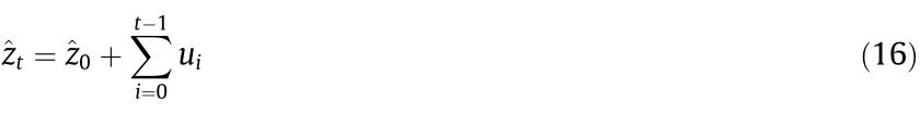
where  is an arbitrary initial point, and the summation term represents the actions taken up to the tth instant (
 = +1 for up, = 1 for down).
Discount factor:  = 0.99.
The goal of this agent is to generate a sequence of actions to overlay the cropping box, B, on the vertical axis of the PSV with the interface at its center. To achieve this, the agent needs to perform long-term planning and preserve the association between its actions and the information obtained from DP cell measurement. A flowchart of the proposed scheme is shown in Fig. 5. In addition, Fig. 6 and Table 2 show the networks in detail. More details about the ConvLSTM layer can be found in Ref. [27].
《Fig. 5》
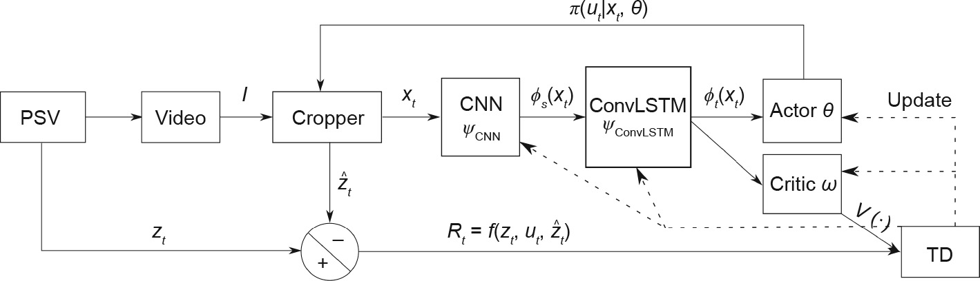
Fig. 5. Flow diagram for the proposed learning process. The update mechanism is shown in Eqs.(9) and (10) with the k-step policy evaluation, as shown in Eq. (14).
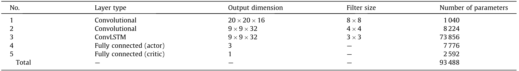
《Table 2》
Table 2 Structure of the global network (the same structure as the workers).
《Fig. 6》

Fig. 6. Detailed structures of the CNN, ConvLSTM, actor, and critic networks.
Unlike the previous works [4,5] that make predictions in the state space, this approach optimizes the value and the policyspaces by using Eqs. (9), (10), and (14), respectively. Moreover, the CNN and ConvLSTM layers are updated by using Eq. (17).

where 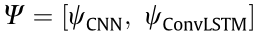 represents the parameters of the CNN and the ConvLSTM layers. This scheme trains the entire network end-to-end by using only the TD error. Multiple workers [48] that are initialized at different points (Fig. 4(b)) can be used to improve the exploration and hence the generalization.
After a suboptimal policy is found, the agent is guaranteed to find the interface in a limited timestep k, independent of the initial point, as shown in Lemma 3.1.
Lemma 3.1: At any time t, for a constant zt, with P = 1,  =0 ,
=0 ,  , as k → N, for
  .
.
Proof. Assume  and the suboptimal parameters
  and
and  are obtained using an iterative stochastic gradient descent over a continuous policy function
  .
.  is a Lipschitz continuous critic network, parameterized by
  , and estimates the value of policy π(∙) for a given state.

This can be extended to a variable  .
.
《3.2. Robustness to occlusion via training》
3.2. Robustness to occlusion via training
CNNs interpret the spatial information by considering the connectivity of the pixels, which improves robustness up to a certain point. However, it does not guarantee robustness to occlusion, and the agent may fail even if a good policy is obtained under normal conditions. To overcome this issue, the agent may be trained using synthetically occluded images during the training phase. Another way is to recalibrate a policy (that was trained using occlusion-free images) with occluded images.
An occluding object, Ω, with an arbitrary pixel intensity,  , can be defined as
  , where
  represents the ratio of occlusion, as shown in Fig. 4(c). If ρ= 1, the agent observes only the occlusion in that video frame (i.e., xt = Ω if ρ= 100%). After defining its size, the ratio of occlusion can be sampled from an arbitrary probability distribution (i.e., continuous or discrete, e.g., Gaussian, uniform, Poisson). During training, the duration of the instance at which the occlusion appears may be adjusted arbitrarily. These can be stochastic or deterministic. That is, the occlusion may appear at a random (or specific) time for a random (or particular) duration. If multiple workers (as described in Section 2.2) are used, different occlusion ratios at different time instances with different durations may be introduced to each worker. This improves the diversity of the training data, which makes the process time efficient, because the agent does not need to wait for a long time to observe different types of occlusion.
《4. Results and discussion》
4. Results and discussion
《4.1. Experimental setup》
4.1. Experimental setup
A lab-scale setup that mimics an industrial PSV is used for the proposed scheme. This setup allows for the movement of the interface to a desired level using pumps, as shown in Fig. 7. Two DP cells are used to measure the interface level based on the liquid density, as described in Ref. [5].
《Fig. 7》

Fig. 7. The experimental setup.
Images are obtained using D-Link DCS-8525LH camera at 15 frames per second (FPS). From the 15 FPS footages, a representative image for each second is obtained. Hence, 80 images from 80 consecutive seconds are obtained with necessary down-sampling. These images are processed to showcase the PSV portion, void of unwanted background. They are then converted into grayscale images. The DP cell measurements (for the same contiguous time period as the images), which are available in terms of water head (water-in), are converted to pixel positions, as given in Ref. [4]. After each action is taken, the video frame changes. Every action the agent takes generates a scalar reward (Eq. (15)), which is later utilized to calculate the TD error (Eq. (14)) that is used in training the agent’s parameters (Eqs. (9) and (10)).
《4.2. Implementation details》
4.2. Implementation details
4.2.1. Software and network details
Both the training and the testing phases were conducted using an Intel Core i7-7500U CPU at 2.90 GHz (two cores, four threads), 8 GB RAM at 2133MHz, and 64-bit Windows using Tensorflow 1.15.0. Unlike deeper networks (e.g., those in Ref. [32] that consisted of tens of millions of parameters), this agent consisted of fewer parameters, as summarized in Table 2. This prevents overparameterization and reduces the computational time significantly, with the disadvantage of an inability to extract higher level features [155].
After each action is taken, the cropping box is resized to 84 × 84 pixels. An Adam optimizer with a learning rate of 0.0001 is used to optimize the parameters of the agent (including the CNN, ConvLSTM, actor, and critic) in a sample-based manner. This momentum-based stochastic optimization method has been reported to be computationally efficient [156].
4.2.2. Training without occlusion
An A3C algorithm was used during the experiments to reduce the training time, improve exploration, and achieve convergence to a suboptimal policy during learning [48]. All of the initial network parameters were sampled randomly from a Gaussian distribution with zero mean and unit variance. Offline training was performed after creating a continuous trajectory of the interface level by manually ordering 80 unique images, as shown in Fig. 8.
《Fig. 8》

Fig. 8. Training results at the end of training (2650 episodes) and FT (3380 episodes). BFT: before fine-tuning; AFT: after fine-tuning.
This trajectory was then repeatedly shown to the agent for 470 steps for 2650 episodes (i.e., an episode consisted of 470 steps). At any time, the agent observed only the pixels within the cropping box. The cropping box of each agent was initialized at four different positions, as shown in Fig. 4(b). The agent’s goal was to minimize the deviation of the center of the cropping box with respect to the DP cell measurements, given a maximum velocity of 1 pixel per step. The agent was not exposed to occlusion during training and was capable of processing 20 FPS (i.e., computational execution time) for four workers.
4.2.3. Fine-tuning with occlusion
The global network parameters were initialized using the parameters obtained at the end of the training without occlusion. The local networks initially shared the same parameters as the global network. All of the training hyperparameters (e.g., learning rate, interface trajectory) were kept unchanged. The images used in the previous training phase were overlayed with occlusion, whose ratio, ρ, was sampled from a Poisson distribution, as shown in Eq. (18). The distribution, Pois(x, λ), is given in Eq. (19).

Eq. (18) bounds ρ between 0 and ρmax = 80% at the beginning of an episode. Shape factor is arbitrarily defined as λ = 1. In each episode, occlusion occurs at the 200th step to the following 200 steps with a probability of 1. The intent behind FT is to make sure the agent is robust to the occlusion. The agent, with four workers, was trained for an arbitrary amount of 730 episodes until the episodic cumulative reward improved.
4.2.4. Interface tracking test
For a 1000-step episode, the agent was tested using a discontinuous trajectory that contained previously unseen images that were either noiseless or were laden with a Gaussian noise,  , in three ways, as shown in Table 3. These images were also occluded using a synthetic occlusion, whose constant intensity was arbitrarily selected as the mean of the image (i.e., κ= 128), while the occlusion ratio, ρ, varied linearly from 20% to 80%.
《Table 3》
Table 3 Definition of noisy images based on their identities.

 represents the Hadamard product.
  is the magnitude of noise.
4.2.5. Feature analysis
To illustrate the effectiveness of the network, a previously unseen PSV image was manually cropped starting from the top of the PSV to the bottom. These manually cropped images were then passed one by one through the CNN prior to training, the CNN was trained as in Section 4.2.2, and the CNN was fine-tuned as discussed in Section 4.2.3 to extract the features. These spatial features,  , were then collected in a buffer with the size 9 × 9 × 32 × 440, from which the reduced dimension (2 × 440) features were obtained using UMAP [99]. These lower dimensional features will be represented in Section 4.6.
《4.3. Training》
4.3. Training
The best policies were obtained at the end of training and FT, when there was no improvement in the cumulative reward for 500 consecutive episodes. Fig. 8 shows the trajectories using these policies. The position of the cropping box is initialized with its center at 60% of the PSV’s maximum height. At the end of this phase, the agent tracked the interface with a negligible amount of offset. An example obtained from the 80th step is shown in Fig. 9(a). The green star represents where the agent thinks the interface is for the current frame.
《Fig. 9》

Fig. 9. (a) Training result at the 80th frame. (b) Test result AFT with 80% occlusion and excessive noise, at the 950th step. The white boxes represent the cropping box that the agent controls. The stars represent the center of the cropping box, and the circles are the exact interface level. The pentagon is the bottom of the occlusion, which looks like the FMI.
《4.4. FT re-calibration for occlusion》
4.4. FT re-calibration for occlusion
FT improved the agent’s overall performance, even for the occlusion-free images, by reducing the level-wise mean average error (MAE) by 0.51%, as summarized in Table 4. This result indicates that the agent adapted to the new environmental conditions without forgetting the previous conditions. This was due to the improvements in the value estimation and the policy, which started from near-optimal points. Note that the minimum value for the MAE is limited by the initial position of the cropping box, as shown in Fig. 8.
《Table 4》
Table 4 Pixel- and level-wise MAE at the end of training and FT.

Fig. 10 shows the cumulative rewards from one of the workers during training and after fine-tuning (AFT), as shown in solid and dash-dot lines, respectively
《Fig. 10》
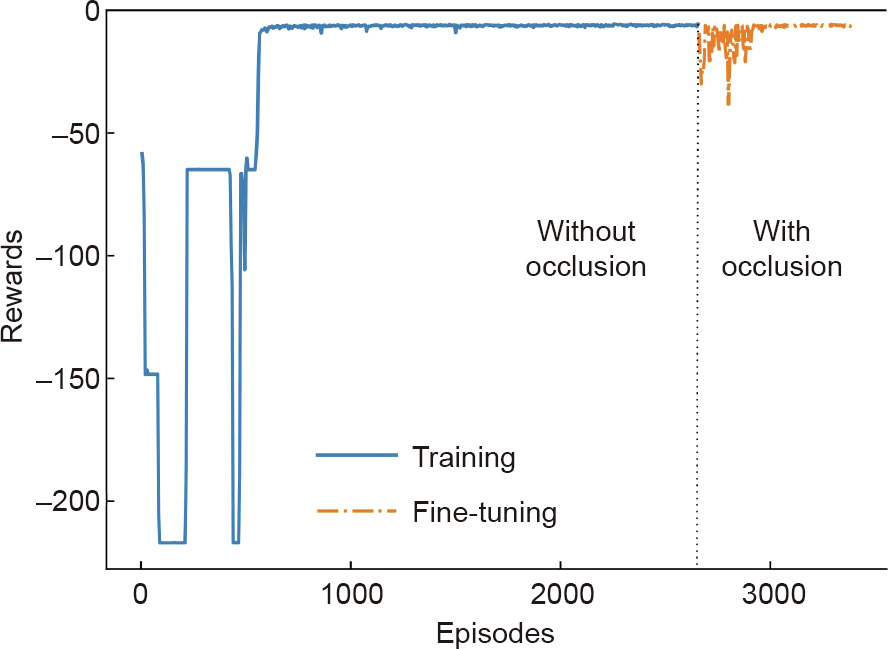
Fig. 10. Cumulative rewards. The graph shows that the agent can learn the occlusion and track the interface successfully.
Note that the initial decrease during FT was caused by the occlusion, because the agent was not able to track the interface level when occlusion occurred. This new feature was learned successfully by the closed-loop reward mechanism within 400 episodes. Note that the final cumulative reward obtained at the end of FT is almost the same as that obtained at the end of training. This is because the cumulative reward represents only the tracking performance during training and depends on the initial position of the cropping box, as shown in Fig. 8. This value can be zero only if the center of the box and the DP cell measurement overlap completely at the beginning of the episode and the agent tracks the interface without any offsets during the episode. The necessity of the FT is more pronounced when the agent is exposed to unseen environ mental conditions such as excessive noise and occlusion, as discussed in Section 4.5.
《4.5. Test》
4.5. Test
4.5.1. Before fine-tuning
The initial before fine-tuning (BFT) test was conducted at the end of the initial training (i.e., the 2650th episode, as shown in Fig. 10). Note that in the testing (online application) phase, DP cell information is not being used, and the RL agent works on its own. In fact, even if the DP cell is available, it will not be accurate in the field application environment. Fig. 11 shows that the agent was robust to up to 50% occlusion and additional noise prior to FT. This is a significant improvement over the existing schemes, all of which do not address occlusion. The reason for this improvement is that the neural networks extract more abstract features than edge and histogram information, in both the spatial and temporal domains [157]. This is due to the convolutional operations that smooth out disturbances and improve the agent’s overall performance. On the other hand, any further increase to the occlusion ratio resulted in failure to track the interface. Since occlusion is of lighter intensity, the policy naturally moved toward the bottom of the PSV (where pixels of higher intensity were abundant) to find the interface.
《Fig. 11》

Fig. 11. Test results: Tracking, where ρ is the occlusion ratio (e.g., ρ = 0.8 means that the image is occluded by 80%).
4.5.2. After fine-tuning
AFT, it was found that recalibrating the agent for occlusion improved its performance significantly, as seen from its ability to track the interface more accurately (Fig. 11). Additional noise caused its performance to degrade when the interface offset between the consecutive frames was around 5%. However, the agent was successful when this interface offset was reduced to 2.5%, as shown in Fig. 11. This is because the excessive noise corrupts the image significantly and the agent fails to locate the interface. An example frame obtained at the 950th frame is shown in Fig. 9(b). It should be noted that the noise is accompanied by 80% occlusion; this makes the tracking problem more challenging, since the amount of useful information extracted by the agent from the image is significantly reduced—that is, only 20% of the pixels can be used to locate the interface. This performance is due to the CNN and ConvLSTM combination. Fig. 12 shows the agent’s beliefs (predicted by the critic) about the states (obtained from an unseen frame) using parameters obtained from a random network (solid), after training (dash-dot), and AFT (dot). According to Eq. (2), this figure defines the value of a state, assuming that the best trajectory toward the interface level would be generated by the policy.
Fig. 12 also shows that, prior to any training, the value predicted for any state is similar. However, during training, the agent regrets being in disadvantegous states, and the DP cell readings reinforce that moving the cropping box closer to the interface (i.e., a vertical solid line) yields a better value than being further away from it. At the end of FT, with more data, the agent further improves its parameters—and therefore its actions—to move the cropper box so that it becomes more accurate. This result shows that the agent tries to improve its actions based on a constantly changing belief (value). Note that the increase in AFT after a deviation value of 200 corresponds to the yellow pentagon in Fig. 9, which looks like the interface and causes an increase in the value function. However, the value obtained from that part is lower than that of the interface, meaning that the agent is more confident when it is close to the star, rather than to the pentagon.
《Fig. 12》

Fig. 12. Test results of value function versus deviation from the interface.
《4.6. Understanding the network: Feature analysis》
4.6. Understanding the network: Feature analysis
The training and test results focused on the progress of the learning and control abilities of the agent. These alone may not be sufficient to explain whether the agent’s decisions are meaningful given an observation in the form of an image.
Fig. 13 shows the reduced dimensionality as a two-dimensional graph by representing the values of the corresponding cropped images (obtained in Section 4.2.5) using the gradual intensities of a color. The curve (from left to right) corresponds to the cropped images from top to bottom of the PSV tank side glass, as explained in Section 4.2.5.
The colored pentagons in Figs. 13(a)–(c) correspond to three points in Fig. 13(d). According to the results, the features obtained from the network prior to training are similar to each other without any particular arrangement. However, as training proceeds, features with similar values get closer. Upon combining Fig. 13 with Fig. 12, it could be inferred that the CNN was able to extract the features in a meaningful way, despite using unlabeled data in a model-free context, due to the RL methodology. This was possible because the texture and pixel intensity pattern of each cropped image was successfully converted into the value and the policy functions by employing a CNN–ConvLSTM combination. Also, the reward signal obtained from the DP cell (which was used as a feedback mechanism) trained the agent’s behavior.
《Fig. 13》

Fig. 13. Dimensionality reduction applied to the features of the states ( ) obtained from an unseen image. The features are obtained using the parameters obtained from (a) random, (b) trained, and (c) fine-tuned networks. The data points are then colored by their corresponding values. (d) Three regions that correspond to the top and the bottom of the tank and the FMI are highlighted on the unseen image. As the agent trains, the extracted features from similar regions are clustered closer in the Riemannian space.
《5. Conclusion》
5. Conclusion
This work provided a comprehensive review on actor–critic algorithms and proposed a novel RL scheme that targets the instrumentation level of the control hierarchy in order to improve the performance of the entire structure. To achieve this result, interface tracking was formulated as a sequential decisionmaking process that requires long-term planning. The agent was composed of a CNN and ConvLSTM combination that does not Fig. 12. Test results of value function versus deviation from the interface. require any shape or motion models and is hence more robust to uncertainties in the process conditions. Inspired from the feedback mechanism used in control theory, the agent utilized readings from DP cells to improve its actions. This technique removes the dependencies on explicit labels that are required for SL schemes. The agent’s performance during validation using untrained images under occlusion and noise showed that the interface can be tracked under up to 80% occlusion and excessive noise. An analysis of the high-dimensional features validated the agent’s generalization of its beliefs around its observations.
《6. Future work》
6. Future work
This work successfully demonstrated the tracking of a liquid interface by utilizing one of the most advanced RL techniques. The occlusion was handled by employing an agent composed of deep CNN structures, and the tolerance was improved by FT the policy, which showcased the adaptive nature of the proposed method. In addition to these, an agent that can reconstruct the occluded images may be an alternative method for future work.
《Acknowledgements》
Acknowledgements
The authors thank Dr. Fadi Ibrahim for his help in the laboratory to initiate this research and Dr. Artin Afacan for the lab-scale PSV setup. The authors also acknowledge the Natural Sciences Engineering Research Council of Canada (NSERC), and its Industrial Research Chair (IRC) Program for financial support.
《Compliance with ethics guidelines》
Compliance with ethics guidelines
Oguzhan Dogru, Kirubakaran Velswamy, and Biao Huang declare that they have no conflict of interest or financial conflicts to disclose.
《Nomenclature》
Nomenclature
Abbreviations
A2C advantage actor–critic
A3C asynchronous advantage actor–critic
ACER actor–critic with experience replay
ACKTR actor–critic using Kronecker-factored trust region
AFT after fine-tuning
BFT before fine-tuning
CNN convolutional neural network
ConvLSTM convolutional long short-term memory
CSTR continuous stirred-tank reactor
DDPG deep deterministic policy gradient
DP differential pressure
FIM Fisher information matrix
FMI froth–middlings interface
FPS frames per second
FT fine-tuning
GAN generative adversarial network
HJB Hamiltonian–Jacobi–Bellman
HVAC heating, ventilation, air conditioning
LSTM long short-term memory
MAE mean average error
MDP Markov decision process
NAC natural actor–critic
PPO proximal policy optimization
PSV primary separation vessel
RL reinforcement learning
RNN recurrent neural network
SAC soft actor–critic
SL supervised learning
TD temporal difference
TD3 twin delayed deep deterministic policy gradient
TRPO trust region policy optimization
t-SNE t-distributed stochastic neighbor embedding
UL unsupervised learning
UMAP uniform manifold approximation and projection
Symbols
 expectation
 spatial features
 temporal features
 temporal difference error
 distribution of initial states
 gaussian noise with zero mean unit variance
 optimum value for the variable, e.g., q*
ln (·) natural logarithm
R, G empirical reward, return
q, r, v expected action-value, reward, state-value
 States
  State space
 Actions Action space
 policy of the agent, also known as the actor
 temporal difference error
V (·) estimate of state-value, also known as the critic
Q (·) estimate of action-value, also known as the critic
Ω occlusion
Parameters
 learning rates for the actor and critic: 0.0001
 discount factor: 0.99
 intensity of occlusion: 128/256
 shape parameter of a Poisson distribution: 1
 occlusion ratio: %
 magnitude of noise: 0.2


 京公网安备 11010502051620号


