《1. Introduction》

1. Introduction

In a smart grid, the contribution of the demand side is key to balancing the grid. Demand response (DR) allows adapting the electricity demand to a varying electricity supply from, for example, renewables. Energy service companies emerge that aggregate the demand of small appliances into volumes that can play a role in an electricity market. This study focuses on aggregators that utilize the flexibility of electric vehicles (EVs), which are charged from the distribution grid. To control its EVs, an aggregator typically determines a collective charging schedule for the fleet, based on the electricity energy prices (economic objective). However, when charging, the EVs are physically connected to a low-voltage distribution grid, which is inherently constrained by its infrastructure. To assure correct operation of the distribution grid, the distribution system operator (DSO) can enforce technical constraints by using grid congestion management mechanisms.

To integrate the objectives of both aggregator (economic objectives) and DSO (technical objectives) in the coordination of EV charging, two operation levels are identified [1,2].

• The market operation level entails actions with the objective of following previously traded volumes on the wholesale electricity markets, where trading takes place on a relatively long-term scale (months, seasons) and amounts are expressed as energy quantities—usually MW•h—in time slots of typically 15 min or 1 h. A time-driven approach is well suited here.

• The real-time operation level entails actions to comply with instantaneous consumer preferences and to respect local grid constraints (such as voltage constraints). Because changes and control are relatively more instantaneous and dynamic at this level, real-time operation (or technical operation) is usually expressed in quantities of electrical power, such as kW. Granularity is in the range of minutes to seconds. At this level, fast response is important and the amount of communication needs to be limited. An event-driven approach is well suited here.

A large part of research on the integration of EVs is aimed at optimally coordinating the charging at the market operation level, facilitating larger shares of renewable energy sources or providing system-wide ancillary services, or minimizing electricity costs for charging [3−5]. At the same time, a considerable amount of the work in literature has been carried out toward the use of EVs to avoid grid overloads or reduce grid losses [6−10], objectives that are situated in the technical operation level.

The interaction between the economic market operation and the technical real-time operation, when coordinating the charging of EVs, has not often been considered [2], except when considered in the same context as vehicle-to-grid energy transfer [11,12]. However, the economic and technical levels can come into conflict, which typically occurs when the distribution grid reaches its constraints (i.e., voltage, current, unbalance, etc.), at which point the technical objectives will intervene in the economic market objective(s). As market operation is overruled, consumption can deviate from what is intended by the aggregator, impacting the aggregator’s business case.

In this paper, the influence of the technical, real-time operation level on the economic market operation level is analyzed by simulating both levels in a set of varying distribution grid scenarios. For the market operation level, an existing event-driven market-based control (MBC) for coordinated EV charging is used. When there is a constraint from the real-time operation level, it will take precedence. In addition, a voltage droop controller can be used to mitigate local voltage limitations. The quantitative effects of using droop control on the aggregator’s objective at the market level will be analyzed.

Section 2 discusses existing algorithms and models for both market and real-time operation levels. Section 3 details and motivates the choice of the algorithm for the market operation level. Section 4 describes a set of relevant distribution grid scenarios, together with an explanation of the models and assumptions for the simulations. In Section 5, the chosen algorithms are simulated in these predefined scenarios, and the influence of real-time operation on market-level objectives is thoroughly analyzed.

《2. Background》

2. Background

《2.1. Market-level operation》

2.1. Market-level operation

Research regarding the optimization and coordination of clusters of DR participants at the economic market level can roughly be divided according to the way in which the optimization is performed, using centralized, distributed, and aggregate & dispatch algorithms (Figure 1).

《Fig. 1》

Fig.1 An illustration of the three classes of algorithms and coordination for demand response (DR) at the market level.

For centralized algorithms, a central actor collects information from the DR devices. This information can consist of individual constraints and deadlines or comfort settings. Using the collected knowledge, and possibly including additional information such as predictions, the central coordinator performs a single optimization that returns an optimal schedule satisfying all the constraints at once. This process inherently makes centralized algorithms less scalable, as the optimization process becomes very computation-intensive with an increasing number of participating devices. Furthermore, the communication to the central actor poses a potential bottleneck. Several solutions are proposed that help to overcome the tractability issue [11,13].

Distributed algorithms, on the other hand, perform a significant part of the optimization process at the participating devices themselves. This way, the computational complexity of finding a suitable solution is spread out over the cluster, typically using an iterative process in which information is communicated between the participants. This distributed aspect does not exclude the existence of an entity responsible for initiating or coordinating the convergence of the iterations. A share of distributed algorithms in literature is based around distributed optimization techniques, in which a large optimization problem is divided into smaller parts that can be iteratively and independently solved [14−17]. In particular, the use of gradient ascent methods and their derivatives, such as dual decomposition, are common.

Aggregate & dispatch algorithms combine both approaches to some extent. They decouple the optimization of the objective from the dispatch of its outcome. An aggregate & dispatch mechanism allows information (such as constraints) from and to the central entity to be aggregated, reducing the complexity of the optimization and improving scalability, but carrying certain compromises or constraints regarding the optimality of the results. The work of Refs. [18−20] follows this idea.

While distributed and centralized algorithms can determine an optimal DR schedule given the appliances’ constraints or market data, they carry some disadvantages regarding computation times, complexity, or communication. Aggregate & dispatch mechanisms are a compromise allowing for a scalable and low-cost implementation with a limited loss of optimality [3]. In this study, MBC is chosen as a particular instantiation of an aggregate & dispatch algorithm (see Section 3).

《2.2. Real-time level and grid congestion》

2.2. Real-time level and grid congestion

As the electricity grid cannot get physically congested, the term “grid congestion” refers to a situation in which the demand for active power exceeds the nominal power transfer capabilities of the grid [21]. Grid congestion can be mapped to the violation of one or more constraints at its connection points. In this paper, these violations will mainly be in the form of power quality problems in distribution grids, and can be attributed to the resistive and unbalanced nature of distribution grids.

2.2.1. Grid congestion metrics

The EN 50160 standard on Voltage characteristics of electricity supplied by public distribution systems describes, among others, the following important specifications.

• Over- and under-voltage: The 10-minute mean RMS voltage deviation should not exceed±10%, measured on a weekly basis. For under-voltages, a wider range is allowed in the measurement procedure: −15% to −10% during the maximum 5% of the week.

• Voltage dip: It allows 1000 voltage dips per year, during which the voltage drops at most to 85% of its nominal value, for a duration of less than 1 min. Interruptions, defined as lasting less than 180 s, should occur fewer than 500 times per year.

• Voltage unbalance factor (VUF): The 10-minute mean RMS value of the VUF should be below 2% for 95% of the time, measured on a weekly basis.

2.2.2. Congestion mitigation

A DSO, faced with grid congestion problems, can opt for a number of mitigating strategies.

• Reactive power and voltage control to increase the (local) transfer capacity: This strategy is already used in wind generators connected to the medium-voltage network. In distribution grids, reactive power and voltage control can be achieved through the use of tap changers and capacitor banks, and their switching is planned using load forecasts. In practice, automated and remotely controllable on-load tap changers are required, but their use in distribution grids is still reserved to a few test cases, due to costs.

• Coordinating the power flow [21] via shifting or curtailing demand: This strategy is possible through the implementation of DR, or through the mandated implementation of mechanisms such as voltage droop control.

• Increasing the transfer capacity of the local grid by replacing or upgrading equipment (adding or replacing cables, installing a bigger transformer, etc.): While this option is attractive because it limits the involvement of the DSO (retaining a passive role with no forecasts, etc.), the cost of this option can be substantial and thus it is only considered when other solutions are exhausted or deemed infeasible.

In this paper, congestion management is considered according to the second option: the coordination of active power demand at congested grid locations via voltage droop control.

2.2.3. Voltage droop control

Distribution lines behave resistively rather than inductively. This characteristic causes voltage deviations along the line when large amounts of active power are drawn from the grid. The voltage deviations can be influenced, as charging rates of EVs can be varied and shifted arbitrarily in time. Thus, in addition to the coordination at the market level, a fast-acting grid-supportive behavior can be implemented inside a charger [22,23]; this implementation can reduce the charging rate in the case of under-voltage situations (or increase it for over-voltage situations). Such a droop control scheme is robust and easy to implement because it only requires the local voltage measurement and a way to adjust local active or reactive power settings. No communication is needed. Figure 2 shows an example of a voltage droop curve for an EV charger. When the voltage at its connection point drops below 0.9 per unit (pu), power is linearly reduced until 0.85 pu, at which point charging is completely halted.

《Fig. 2》

Fig.2 An example of voltage droop control characteristic for electric vehicle (EV) chargers.

On the downside, the activation of the droop at the technical operational level will affect and influence the economic market-level coordination [24]. For example, at some point the aggregator will send its optimal power set points or an equilibrium priority to the vehicle agents, but due to local grid problems, the charger may be forced to reduce power; this situation can result in a deviation from the optimal market-level energy plan, and a potential penalty for the aggregator.

《3. Market-level operation: MBC for EVs》

3. Market-level operation: MBC for EVs

The concept of MBC is rooted in microeconomics, wherein economic activity is modeled as an interaction of individual parties pursuing their private interests [25]. The market mechanisms that apply provide a way to incentivize the parties, referred to as economic agents, to behave in a certain way. In Ref. [26], appliances in a DR cluster are represented by software agents in a multi-agent system (MAS). They have control over one or more local processes (e.g., heating water or charging an EV’s battery), but they compete for resources (electric power) on an equilibrium market with other agents.

《3.1. Architecture》

3.1. Architecture

The MBC system has been used in a number of field tests and is commercially known as PowerMatcher. The clearing of the market in Refs. [26,27] is operated on a periodic basis (e.g., a time-slot length of 15 min) or using events, and is implemented in a hierarchical, tree-like manner [25].

At the top of the hierarchy is an auctioneer agent that is directly connected to a number of concentrator agents. The auctioneer agent is a special type of concentrator agent and is responsible for the price-setting process, just as in Walrasian auctions. The concentrator agents lower in the hierarchy aggregate the demand functions of their child agents. Because a uniform interface is used between the levels, an unlimited number of such aggregation levels can be used. Eventually, at the bottom of the hierarchy, the device agents themselves are found.

The device agents assemble demand functions representing their willingness to pay and consume electricity, taking into account the specific constraints of the controlled device. Demand functions are sent upwards and an auctioneer agent performs a matching process with producing agents. An equilibrium price is communicated back to the agents, which start consuming or producing at the equilibrium level. This process is illustrated in Figure 3.

《Fig. 3》

Fig.3 (a) An overview of the control structure in MAS MBC; (b) demand functions P_demi, as sent upwards by device agents from charging EVs; (c) after aggregation of the individual demand functions, equilibrium priority p_equi is determined and sent back to the agents.

If equilibrium prices are regarded as a pure control signal, so that there is no direct link to the cost of energy, the MAS MBC mechanism can be viewed as a dispatching method for the aggregator’s business case. In such a scenario, the demand function data is regarded as input for a scheduling algorithm, and the equilibrium price (or better, the equilibrium priority) is regarded as a signal to steer the cluster toward its outcome.

3.1.1. Demand functions for EV device agents

Representative demand functions can be built using various means, but in the case of EVs, a straightforward way is by combining each agent i’s requested energy ⁱE_req, time till departure ⁱΔt_dep, and maximum charging power ⁱP_max⁡ to create a sloped curve ⁱP_dem (Eq. (1)), as is shown below each EV in Figure 3(a) and (b). In case there is not enough time left to receive the requested energy (i.e., t_critical occurs before the current time), an inflexible demand function can be used, so that charging happens at maximum power regardless of the control signal (Eq. (2)).

A detailed description of building demand functions for EVs in this context can be found in Refs. [2,3].

3.1.2. Concentrator agents and aggregation

At the level of the concentrator agents, the individual demand functions of n agents are aggregated into a single curve (Eq.(3)), shown in Figure 3(c). At the auctioneer agent, this aggregated curve is used to find the equilibrium priority p_equi that corresponds to a desired power setting P_ctrl for the DR cluster (Eq. (4)).

The value for P_ctrl is determined by the business agent.

《3.2. MAS MBC advantages and drawbacks》

3.2. MAS MBC advantages and drawbacks

Using a MAS MBC system for DR, as exemplified by the PowerMatcher, offers several benefits.

• Scalability: In a centralized system, the central entity has to deal with all incoming and outgoing messages, O( n), quickly creating a communication bottleneck. Because of the aggregation on multiple levels in the PowerMatcher, the quantity of messages that must be dealt with per agent can be reduced to O(log n).

• Low complexity: The construction of demand function data and the matching process itself is straightforward, and is not based on any model. Determining a demand function for a device can be done during its development.

• Openness: Any kind of device can be integrated in the cluster, since operation only depends on the exchange of demand functions and price. Devices without flexibility are represented by an inelastic demand function.

• Privacy: Since demand functions are aggregated, there is no central entity that collects all information. Furthermore, the physical processes of devices, bidding strategy, and motives of users are all abstracted through their demand functions.

However, a more significant shortcoming of the original PowerMatcher approach is the lack of look-ahead functionality.

《3.3. Addition of scheduling functionality and control objectives》

3.3. Addition of scheduling functionality and control objectives

For loads that can store electric energy, such as EVs, an energy constraints graph can be used to capture the available flexibility over a certain time horizon. This graph is introduced in the work of Ref. [3]. For each EV i, two vectors ⁱE_max⁡ and ⁱE_min are added to the information ⁱP_dem sent from device agents to the auctioneer agent (Eq. (5)).

The vector ^⁡iE_max is the energy path of an EV agent i, if it must start charging immediately at maximum power and then (at t_idle) stay idle until its departure time t_dep. On the other hand, ^⁡iE_min represents a case in which charging is postponed for as long as possible (up to t_critical). These situations are expressed in Eq. (5) and illustrated in Figure 4(a). All of the area between ^⁡iE_max and ^⁡iE_min⁡ represents the flexibility of the charging process.

《Fig. 4》

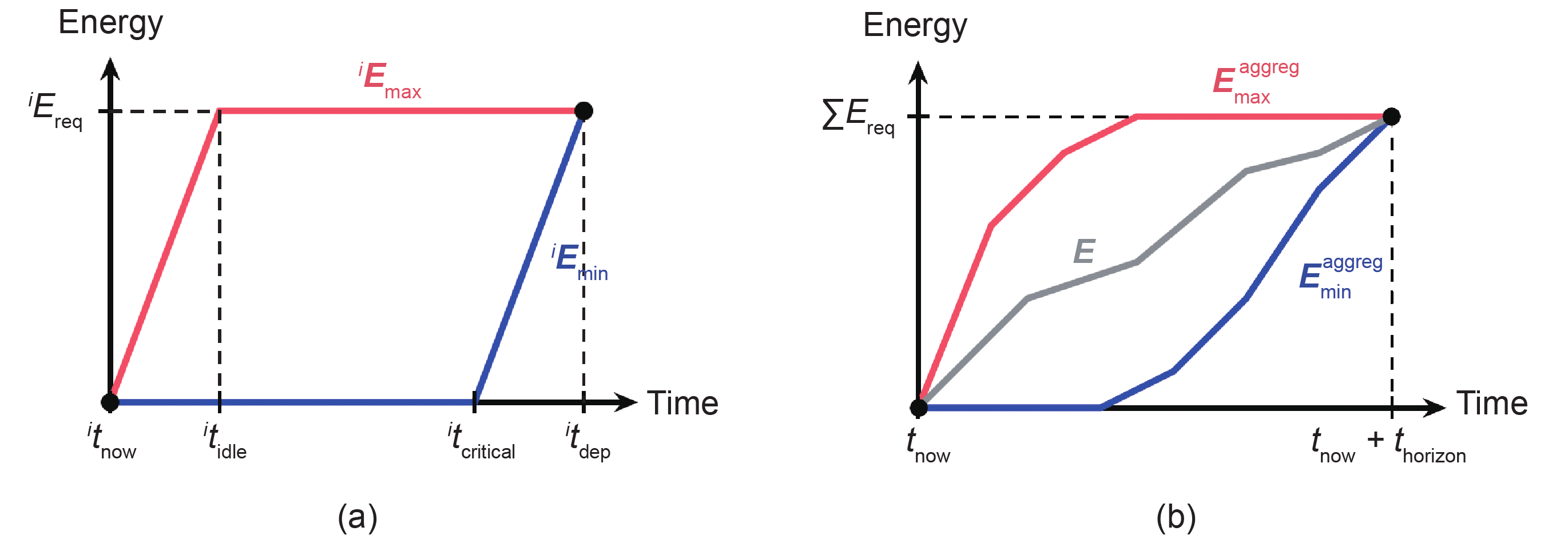
Fig.4 (a) An energy constraints graph for a single vehicle i; (b) an aggregated energy constraints graph and some scheduled path E through it.

To represent the battery constraints of an entire EV fleet of n vehicles, the individual constraints are aggregated into collective battery constraints and , at the intermediate agents and at the auctioneer agent. The auctioneer agent can now use the collective energy constraints to determine an optimal path E_opt over the horizon t_horizon, according to some objective function C (Eq. (6)):

where E_t is the collective energy of the cluster at time t; and P_t is the power consumed by the cluster during time t to ∆t. Any objective C( E) can be used to determine a path for the EV cluster; Section 4.1 discusses two such objectives.

《4. Simulation objectives and models》

4. Simulation objectives and models

A situation was investigated in which an aggregator coordinates a cluster of EVs based on market-level objectives, but a large part or all of the vehicles are situated inside a weak and constrained distribution grid. Different questions arise, such as

• How effective is the use of a voltage droop controller in eliminating or reducing grid congestion problems?

• To what degree do such technical objectives impact the aggregator’s business case?

To answer these questions, a simulation framework was developed. A Java-based part of the framework allowed the interaction between the agents to be modeled, while the market-level optimization was performed in Matlab using CPLEX. To simulate the effects on the voltages in a distribution grid, a Matlab-based backward-forward sweep load flow solver was integrated into the framework. In addition to a framework, several models and datasets were required in order to properly represent the actors and their behavior.

《4.1. Aggregator market-level objectives》

4.1. Aggregator market-level objectives

Two market-level objectives for the auctioneer agent were considered.

• Time-of-Use (ToU), in which the aggregator’s goal is to minimize the cost of charging a cluster of vehicles, based on a time-varying tariff p_t, and using a linear program (LP) optimization (Eq. (7)):

Because this is a linear objective, an on-off control behavior of the EVs can be expected.

• Portfolio balancing, in which the goal of the aggregator is to use the EV flexibility to limit its portfolio’s wind generation exposure to the imbalance markets. This goal means finding an optimal energy trajectory for the EVs, E_EV, over a horizon, such that the difference between the short-term prediction E_wind of wind energy and its day-ahead nomination E_nomin is minimized (Eq. (8)):

In this specific case, the day-ahead nominations are required to be supplied on an hourly basis, while the short-term wind power predictions are known on a quarterly basis (15 min ahead), and with a horizon of 24 h, as shown in Figure 5. The control variables of the EVs can be on an arbitrary time basis.

《Fig. 5》

Fig.5 An illustration of the balancing obj­ective.

Thus, as more accurate wind power predictions become available after the nomination, the optimization will try to use the EVs to limit the difference, and, due to the quadratic term, will favor spreading out the remaining imbalance over the period of time until the considered time horizon.

《4.2. Models for EV, wind power, and loads》

4.2. Models for EV, wind power, and loads

The model of the (plug-in) EVs in the simulations consists of two main parts: a battery model and a usage or driving profile.

• All EV instances are equipped with the same usable battery content of 20 kW•h. This content corresponds, for example, to the 10% and 90% state-of-charge of a 25 kW•h battery. It is assumed that vehicles want their usable battery content fully charged by the time of departure.

• Charging takes place at a variable power level between 0 and 3.3 kW from a single-phase connection of the distribution grid.

• Data about the state of the vehicle during the day (i.e., idle at home, driving, unavailable, etc.) and the energy consumption while driving is taken from Ref. [28].

• Data for renewable energy production from wind turbines is based on Ref. [29] and adapted to a 2.5 MWp turbine.

To be able to simulate their effects on voltage quality in a distribution grid, realistic household consumption profiles are required. Profiles from the “Linear” smart grid project [30] were used, which are based on measurements at 100 households for one year, with a resolution of 15 min.

《4.3. Weak grid topology and agent architecture》

4.3. Weak grid topology and agent architecture

When investigating the effects of coordinated charging on the state of the distribution grid and vice versa, it makes sense to focus on weak grid configurations, for which problems are more likely to occur.

Figure 6 shows the base topology used in the simulations. A 400 kVA transformer supplies several parallel feeders. Each feeder then supplies a number of household loads, bringing the equivalent transformer load up to 191 households. One of the feeders, Feeder 0, is linked to a line-segment supplying 38 single-phase household connections. These connections are alternatingly attached to phases 1 to 3 and spaced apart by distance D2. The distance from the transformer to the first household connection is D1. From each connection point, a cable with length D3 runs from the line to the household’s supply terminals. In the simulated model, the other feeders and loads (153 households) connected to the transformer are lumped together into one single entity (Feeder 1), as their impact is not studied in detail.

《Fig. 6》

Fig.6 (a) A single instance of the physical grid topology; (b) agent topology in relation to the physical grid.

Cable parameters are taken from the design specifications of underground distribution cables, NBN C33-322. Cable type EIAJB 1 kV (3 mm × 70 mm+ 1 mm × 50 mm) is used for the main feeder and line (D1, D2), while cable type EXVB 1 kV (4 mm × 16 mm) is used to connect the household’s supply terminals to the main cable (D3).

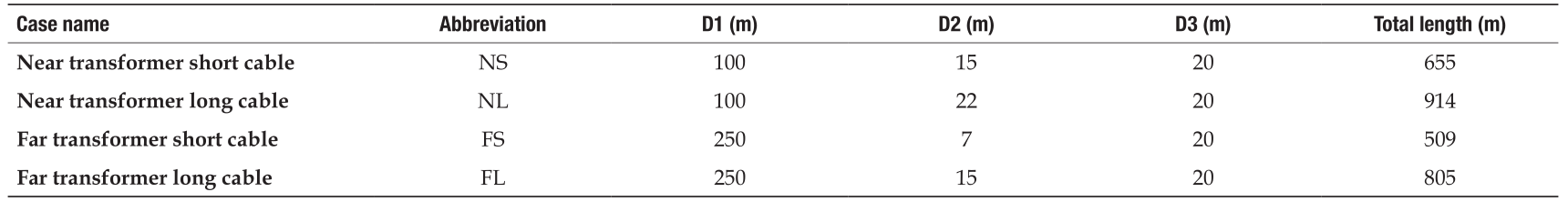
Table 1 shows the variations on this topology that are evaluated in the next sections. Cases NS and NL have a relatively short cable between the transformer and the first household terminal (100 m). Cases NL and FL represent scenarios with rather long total cable lengths (914 m and 805 m), due to longer distances between the household connection points.

《Tab.1》

Tab.1 Variations of the physical base topology, representing various weak grids.

The organization of the software agents representing the charging vehicles, shown in Figure 6(b), is independent of the grid topology. However, it is assumed that all agents for vehicles that are physically connected to the same transformer are grouped under a single concentrator agent. At the same time, in order for the market operation at the aggregator to function properly, more flexibility should be available in the cluster than what is provided by the 38 vehicles in the base topology. To that end, the cluster is extended so that, depending on the scenario, a total of 200 or 1000 vehicle agents take part in the coordinated charging. These additional agents are not part of the load flow calculations.

To test additional shares of EVs inside weak distribution grids, additional variations of the agent structure are created by having multiples of the base topology. These multiples are shown in Table 2. The suffix after the case number determines the share of agents used in the topology.

《 Tab.2》

 Tab.2 Variations of the agent topology, representing different quantities of vehicles situated in weak grids.

《5. Aggregator cases: Simulations and results》

5. Aggregator cases: Simulations and results

This section examines the effect of coordinated charging using market-level objectives on local grid congestion, in the distribution grid scenarios from the previous section. In addition to the MAS MBC event-based implementation that was outlined before, an uncoordinated (dumb) charging scenario is included, during which vehicles plug in and start charging upon arrival at their maximum rated power P_max.

The first set of scenarios deals with an aggregator that tries to minimize the cost of charging a fleet of EVs when a particular ToU tariff is given (Section 5.1). The second set of scenarios considers an aggregator that has to balance its portfolio when deviations from the day-ahead market occur because the portfolio contains wind generation (Section 5.2).

In both sets, the technical constraints are discussed as real-time level results, and the economic aspects are discussed as market-level results.

《5.1. Aggregator with ToU cost objective》

5.1. Aggregator with ToU cost objective

The objective of the aggregator during a ToU scenario is to respond to a 24-hour horizon ToU tariff in such a way as to minimize the charging cost of the vehicle fleet. The 24-hour tariff in this scenario is based on the wholesale energy price of the hourly Belgian BELPEX day-ahead market.

Because of the seasonal effects of household consumption and tariffs, distribution grid problems are correlated to the time of year. To limit the influence of the choice of day on the results, and in order to get a global picture, randomized sets of scenario parameters were generated and tested. The randomized parameters include the day for which the tariff is selected, the vehicle driving profiles, and the household load profiles. Results for voltage problems according to the EN 50160 standard are shown for 100 randomized parameter sets per case.

The different scenarios sample the problem space according to several dimensions:

• Physical grid topology, representing different weaknesses of the grids (NS, NL, FS, FL);

• EV penetration, representing different shares of EVs ( x-38, x-114, etc.); and

• Coordination techniques (household-only (HHOnly) = reference case without EV, Dumb= uncoordinated charging, Event= MBC only considering cost objectives, Event+ droop= considering both economic and technical constraints).

5.1.1. Real-time level results

Looking at the HHOnly results in Figure 7, it is clear that the chosen topologies work well as long as no EVs are introduced. When EVs are charged in an uncoordinated way, the voltage problems are outside the EN 50160 specifications by a wide margin, confirming that the grid topologies qualify as “weak grid.” Voltages regularly drop below 0.9 pu for more than 5% of the time, as shown in Figure 7(a), and events during which the voltage drops below 0.85 pu, as shown in Figure 7(b), are quite common. In addition, too many unbalances occur between the phases, as shown in Figure 7(c). These problems would become even worse in situations with unbalanced phase connections, higher charge currents, and increasing household loads.

《Fig. 7》

Fig.7 EN 50160 voltage magnitude and unbalance problems over the course of seven days, for 100 randomized days. (a) Voltage below 0.9 pu; (b) voltage below 0.85 pu; (c) VUF greater than 2%.

Still, the severity of distribution grid problems strongly depends on the grid topology, shown as cases NS, NL, FS, and FL. Case FL has the longest cable sections to the loads, leading to the highest voltage magnitude and the most VUF problems, while cases NS and FS experience the fewest problems.

However, the observed trend is the same: Uncoordinated charging is responsible for a peak in the evening that overlaps with the peak of household loads. Basing the charging coordination only on ToU cost minimization leads to fewer voltage problems; however, too many voltage problems still remain. The reason for these continuing problems is that, although the coincidence of household loads and charging has disappeared, all available vehicles are now asked to commence charging at one or two points during the day. This synchronicity creates a new peak that is sufficient to create voltage problems. When voltage droop controllers are used, the severity of the voltage deviations is reduced. However, because the voltage droop control only activates below 0.9 pu, the measured values for 0.9 pu deviations are still frequently outside the 5% specifications of the EN 50160 standard. Issues related to voltage below 0.85 pu are solved entirely. By tuning the set point of the controller so that it intervenes sooner (e.g., at 0.95 pu), the weak grids can be brought into full EN 50160 compliance.

5.1.2. Market-level results

Table 3 shows the cost of charging for a cluster of 200 EVs. Due to technical constraints, the eight cases were simulated in separate batches. Because different random parameter sets were generated for each batch, the total cost values between the cases cannot simply be compared.

《 Tab.3》

 Tab.3 Cost results for the ToU scenarios, and the difference due to the use of voltage droop control in the EV chargers; the cost difference due to the undelivered energy is also shown.

During droop control intervention, some vehicles can end up with an incompletely charged battery at the time of departure t_dep. Since this result influences the cost numbers, a cost must be attached to the resulting energy deficit. E_deficit equals the difference between the requested battery level and the level at which the vehicle departed (Eq. (9)):

A cost of €50 (MW•h)⁻¹ is assigned to this energy deficit. Of course, the amount of deficit is directly related to the number of vehicles that can suffer from distribution grid problems. Vehicles outside of weak distribution grids will obviously never end up with lost energy.

While the droop controller has a positive effect on the occurrence of voltage problems, it also increases the cost of charging the fleet, as more energy is consumed during unfavorable periods. Without taking into account the energy deficit at departure time, there is already a small cost increase of 0.6% for the x-38 cases, and of almost 2% for the x-114 cases, in which close to 60% of the EVs are situated in weak distribution grids. Taking into account E_deficit, this cost increase is doubled, and the cumulative battery deficit volume takes up to 1.15% of the total delivered energy.

5.1.3. Conclusions on the ToU scenario

From the results, it is apparent that ToU-based controlled EV charging has the potential to create significant power quality problems, because of the tendency to synchronously switch large amounts of controlled loads when market prices are low, thereby creating large power peaks.

The effect of ToU-based optimizationon on the state of the distribution grid can be even worse than when no coordinated charging is used (dumb charging). In fact, the situations contained two particular mitigating factors: The household connection points’ phases were alternatingly distributed along the line, and the price profiles used by the aggregator kept the power peak of the vehicles out of the household’s evening peak. If these two factors were not present, the EN 50160 results would be worse.

On the positive side, the use of a simple voltage droop controller practically solves all the encountered power quality issues and is able to bring relatively weak distribution grids back into EN 50160 compliance, with some tuning. However, the use of a droop controller has a negative impact on the business case of the aggregator, as the cost of charging goes up and a small number of vehicles do not get their required charge at departure time. However, quantitatively speaking, the differences only start to become significant (>2%) when a large share (>50%) of an aggregator’s fleet is situated inside weak grids.

《5.2. Aggregator with balancing objective》

5.2. Aggregator with balancing objective
In the previous section, the objective for coordinated charging at the market level was the cost of charging for the whole fleet, taking into account a ToU tariff for the upcoming 24 h and the constraints of the vehicles.

Alternatively, an aggregator could use the flexibility of a fleet to reduce the uncertainty in its portfolio after day-ahead commitments are made, in order to limit its exposure to the balancing market. In Europe, balancing services are traded on separate markets than wholesale energy [31]. While the prices for these services are correlated to those of the energy markets, they tend to be higher. The responsibility and the costs of balancing are usually attributed to an access-responsible party (ARP), which will prefer to reschedule its own generation portfolio rather than being exposed to the balancing market.

For wind farms, for example, wind power predictions are used to build estimated production profiles and the required day-ahead nominations. Since the predictions are not perfect, real output will deviate from the day-ahead prediction during the day itself, and without intervention this difference leads to a positive or negative imbalance, with associated costs. By using the energy flexibility of the charging vehicles, an aggregator can reduce this wind imbalance.

It is assumed that the wind farm is not directly connected to the distribution grid to which the EVs are connected; that is, only the active power aspects of the wind generation require balancing by the EVs, and the voltage profile is not affected by the wind power plant.

The main difficulty in compensating for wind power prediction errors with EVs, however, is that large imbalances require the shifting of a considerable share of the fleet’s available flexibility. Because the driving behavior of a fleet has a 24-hour periodicity and remains relatively constant over time, the amount of charging energy per day shares the same characteristics. Additionally, wind power prediction errors do not cancel out over a day, but persist for longer time periods. Therefore, using all the EV flexibility early in the day means that later imbalances can no longer be compensated for. A possible solution consists of incorporating stochastic optimization and intra-day prediction updates to refine the scheduling process.

A similar reasoning can be considered in order to balance the variability of photovoltaic or other renewable distributed energy resources.

Another possible source of imbalance lies in the time resolution of the nominations; nominations for the day-ahead market in Belgium require energy values on an hourly basis. However, imbalance volumes are settled on a 15-minute basis. Even if an ARP has predictions on its portfolio with high resolution and accuracy, an imbalance will still occur, as nominated values are averaged per hour. The description of this optimization problem was provided earlier in Section 4.1 (Eq. (8)). The nominated energy E_nomin consists of a nomination for the EV fleet and the day-ahead wind power prediction with a resolution of 1 h, for 24 h (Eq. (10)).

Such nominations have to be determined by the ARP or aggregator; for example, by using historical records or estimates. Because the driving behavior of an entire fleet (if large enough) is stable and predictable, it can be justifiable to use the power profile of a previous day or week as the nomination for the fleet.

When historic energy constraints graphs are used, the amount of flexibility at any given time can be maximized by following an energy path through the graph according to a fixed ratio of, for example, 1/2 or 1/3 between  and . Figure 8 illustrates such a planned path. The power values that correspond to the path can then be translated to hourly energy values in order to compose E_{EV,nomin, t}.

《Fig. 8》

Fig.8 An example of EV nominated energy based on historic aggregated energy constraints data.
An extra decay term, γ, can be added to reduce the influence of long-term information in the objective function (Eq. (11)).

A γ<1 will assign a higher optimization cost to the quarter-hour imbalance values that are closest in time. In the limit, a γ→ 0 will mean that the system will behave myopically, as no information about the future is taken into account. The system behaves according to the MAS MBC algorithm without planning, and minimizes the instantaneous imbalance.

In order to evaluate the benefit of using this objective, a new “dumb” scenario is added during which the aggregator only attempts to keep the energy consumption as close as possible to the nomination (referred to as tracking the nomination with the fleet). All scenarios use the event-based MAS MBC system to coordinate the fleet, but in the tracking scenario, no optimization to minimize the difference with the nomination using short-term wind power data takes place.

5.2.1. Simulation scenarios and performance metrics

Due to the relatively long simulation times, the need to prepare nomination data for the wind and EVs, and an exponentially increasing set of parameters, a fixed simulation case was chosen for the simulations. A case was chosen in which the wind power and vehicle profiles for one week start at a particular day in the dataset, in order to include a week during which the first three days had relatively little wind power imbalance and the last three days had a relatively large imbalance. To end up with a significant amount of energy flexibility, the EV cluster consists of 1000 vehicles, rather than 200 as in the previous case. Similar to the ToU scenarios above, situations were selected in which different shares of the vehicles were inside weak distribution grids (Table 2).

The main performance indicator consists of the total energy volume of the remaining quarter-hour imbalance and the resulting cost, based on market data on the positive and negative imbalance price from the Belgian market in 2012.

Unless the ratio of energy flexibility to wind power is very high, it is difficult to end up without imbalance under high wind power conditions, when predictions are difficult. However, the quadratic nature of the objective will favor the spreading out of the imbalance as much as possible, so that a relatively flat imbalance profile should be obtained in the case of γ = 1. Therefore, looking solely at the remaining imbalance volume as a measure of performance does not capture the intent of the algorithm’s objective. In fact, a myopic algorithm, instantly matching imbalance figures with EV flexibility, will perform better in reducing the remaining imbalance volume.

Because the ability to smooth or influence the occurrence of imbalance can be very beneficial for an ARP, it makes sense to look at the variability of the imbalance profiles. The spectral content of the imbalance profile is obtained by taking the sum of Fourier transformations over a sliding window of 32 profile samples. Next, the mean value is subtracted in order to get rid of the DC component, and the area under the spectral plot is retained, expressed in kW Hz. The higher this value, the more variability exists on the power profile of the remaining imbalance.

To evaluate the effects at the real-time level, the EN 50160 specifications and performance indicators from the ToU case were used here as well.

5.2.2. Market-level results

In the first simulation, only the behavior at the market level was investigated, disregarding the distribution grid completely. In Figure 9(a), the 15-minute imbalance volumes are plotted for different values of γ, for a simulation covering seven days. It is apparent that the event-based balancing successfully reduces the amount of imbalance with the nomination. Smaller γ values lead to the aforementioned myopic behavior and force the imbalance profile close to zero, until the aggregator runs out of short-term flexibility.

In Figure 9(b), the Fourier-transformed imbalance volume is plotted. Thus, this figure includes frequency components of the imbalance volume. In the case of the balancing optimization scenarios, it is apparent that imbalance profiles contain fewer high-frequency components than when no balancing optimization is done. This observation confirms the result that can be seen in Figure 9(a), namely that the case with the balancing optimization for γ = 1 is better able to spread out the remaining imbalance than for smaller values of γ.

《Fig. 9》

Fig.9 (a) An imbalance scenario, with the remaining imbalance profile for different values of γ over the course of seven days and for a peak wind power output of 1.25 MW ( W = 0.5), together with the tracking scenario; (b) a spectral plot of the power profiles, expressing the variability of the remaining imbalance.

In the above scenario, the wind power nominations and measurements were scaled with a factor W = 0.5, in order to obtain a peak wind power output of 1.25 MW. Varying ratios of wind power and vehicles were also examined, and the results are shown in Table 4.

《Tab.4》

Tab.4 Balancing case simulation results for seven consecutive days and a cluster of 1000 EVs, for different values of the wind power scaling parameter W and discount factor γ.

The improvement in the remaining imbalance volume over the tracking case is between 20%−30%. Smaller γ values lead to a slightly smaller imbalance remaining over seven days. However, since the objective of the optimization is related to the quadratic imbalance over the optimization horizon, the conclusion that a myopic algorithm performs better based on the total remaining imbalance would be misleading. This conclusion has to be considered along with the “spreading” of the remaining imbalance, which is expressed by the spectral content in the “Volume difference” column of Table 4.

For larger wind power scaling factors, and thus larger wind power prediction errors, the improvement in the remaining imbalance decreases to 16%−21%. A similar effect is observed for the spectral content values. It can be deduced that, based on this balancing method, 1−1.25 MW of wind power can be properly compensated per 1000 EVs. Higher or lower shares of wind power decrease the efficiency of this system.

5.2.3. Real-time level results

For the effects at the distribution level, the different scenarios come into play again. From the tested parameters in the previous section, the wind power scaling is kept at W = 0.5, since this parameter led to the best performance at the market level, and γ = 1, as this is the most generic application.

The EN 50160 results of the passive distribution grid scenarios are grouped together with the active distribution grid scenarios in Figure 10, in order to improve clarity and avoid duplication. These plots show the results for the FL case, but the HHOnly results have been omitted, since their results are the same as in the previous section.

《Fig. 10》

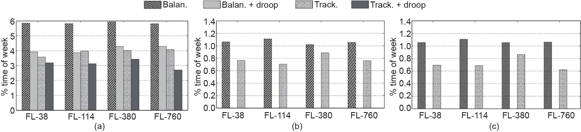
Fig.10 EN 50160 voltage magnitude statistics for the aggregator balancing scenarios. (a) Voltage less than 0.9 pu; (b) voltage less than 0.85 pu; (c) VUF greater than 2%.

Compared to the ToU results, fewer problems exist, but voltages still drop below 0.85 pu. The use of voltage droop control reduces the few remaining voltage problems to below the EN 50160 specifications.

Since the tracking scenario already attempts to follow the nomination, which is a smooth path through the aggregated energy constraints graph for the EVs, the reduction in voltage deviations is relatively small when voltage droop controllers are introduced.

5.2.4. Impact of droop control on market-level objectives

The vehicles for which charging is affected by voltage droop activation will influence the business case at the market level. It follows that moving from case FL-38 to FL-760 will increase the remaining imbalance, as less peak flexibility is available to the aggregator. Figure 11 shows that the imbalance volume is constant for cases FL-38 and FL-114, which have 4% and 21%, respectively, of all EVs inside a weak grid.

《Fig. 11》

Fig.11 Total remaining imbalance after seven days, for different shares of EVs in weak distribution grids. With larger shares, an effect on the remaining imbalance is noticeable, as the aggregator fails to compensate for the droop controller activation.

For case FL-380, with 38% of the fleet inside the weak distribution grids, a small increase of 2.4% in the imbalance volume is noticeable. Finally, for case FL-760 in which 76% of the EVs are located inside the constrained grids, the observed increase in the imbalance volume is 10.3%. During the latter case, the “dumb” tracking scenario also suffered slightly, with a minor increase of 0.95%.

The use of a voltage droop controller in the balancing optimization case leads to fewer and smaller power peaks, as shown in Figure 12. There is practically no gain for the tracking scenario, which attempts to accurately follow the day-ahead nominated EV energy.

《Fig. 12》

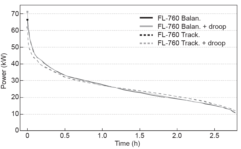
Fig.12 The load duration curve for the FL-760 balancing scenario, for Feeder 0.

5.2.5. Conclusions on the balancing case

The balancing concept was successfully tested on a portfolio consisting of wind power generation and charging EVs. The optimization reduces both the imbalance that originates from the hourly discretization of the day-ahead nomination and the imbalance that exists because of imperfect wind speed predictions. Using short-term information on wind power production, the imbalance can also be intentionally spread over a period of time. This can be beneficial for the aggregator, as the remaining imbalance can then be countered by the other generation units in its portfolio.

In addition, the effect of varying the discount factor γ was shown. By including γ as a variable in the optimization, it was possible to move the remaining imbalance toward points in time in which it had economic benefits, such as by using stochastic information on the imbalance market prices.

Regarding grid constraints, the use of the (quadratic) balancing objective puts less load on the grid compared to the (linear) ToU objective, because the flexibility of the EVs is intentionally spread out when creating the nomination of the charging energy and is therefore not enabled all at once.

As in the ToU case, voltage droop controllers inside EV chargers are successful in mitigating weak grid problems. Some tuning of their parameters may be needed in order to find a setting at which the grid state at all nodes is within the EN 50160 specifications for the entire simulated time.

Unless a very large share of the EVs of an aggregator is located inside weak grids, the business case is practically unaffected by the addition of local voltage droop control, using the coordination system that was implemented in this study. The suggested best choice is to be event-based for fast response, and to have a compensation loop at the aggregator. The combination of both ensures that, when droop controllers activate, the equilibrium priority is changed quickly enough such that the flexibility of the other vehicles is dispatched in order to compensate for the expected energy that is not supplied to the EVs over time.

《6. Conclusions》

6. Conclusions

In light of the challenges that were discussed in the introduction, the results and contributions can be summarized as follows:

• The separation between two DR operation levels has been identified. The market operation level is responsible for the business case of a fleet of EVs and operates synchronously with the energy markets. The technical or real-time operation level uses the set points determined by the business case and uses an event-driven architecture to efficiently dispatch constraints from and control signals to the charging EVs. At the market level, an algorithm based on MBC has been adapted for the coordination of EVs—taking future flexibility into account—and at the technical level, a voltage droop controller has been integrated in order to respect the local grid constraints (mainly under-voltage).

• The effect of using market-level objectives on congestion in weak distribution grids has been examined. In particular, the use of ToU cost minimization objectives has a negative effect on the occurrence of under-voltages, with respect to the EN 50160 standard. The synchronization of large amounts of controllable loads is to be avoided in DR applications.

• In addition to a ToU cost minimization objective, it has been shown that a cluster of fast-responding EVs can be used to limit an aggregator’s exposure to the balancing market. An optimization at the market level determines set points for the fleet such that the remaining imbalance between predicted and nominated wind output and more recent short-term predictions is spread out over a period of time. This can be beneficial for the aggregator, as the remaining imbalance can be then be countered by other generation units in its portfolio. In addition, a variable γ can be included in the optimization in order to express a preference for having the remaining imbalance occur at a time for which it has cost benefits.

• A straightforward and common way of mitigating grid congestion is the use of a voltage droop controller. Although it is fast, inexpensive, and able to act independently from any central coordinator, its activation intervenes in the business case. In literature, the overruling of the market operation level by technical objectives is often presented as a major challenge to be addressed. The results from Section 5 show that, unless very large shares of the EV fleet are located inside weak grids, the effects of the activation of voltage droop controllers on the business case remain relatively modest. These modest effects are due to the limited amount of scheduled energy that is not supplied to the EVs and to the possibility to compensate for this energy using other parts in the DR cluster, based on the event-driven approach.

《Acknowledgement》

Acknowledgement

This project is supported in part by the European Commission through the project P2P-Smartest: Peer to Peer Smart Energy Distribution Networks (H2020-LCE-2014-3, project 646469).

《Compliance with ethics guidelines》

Compliance with ethics guidelines

Geert Deconinck, Klaas De Craemer, and Bert Claessens declare that they have no conflict of interest or financial conflicts to disclose.