
《1. Introduction》
1. Introduction
With progress in computer science and technology, structural optimization design has become one of the most important means of obtaining light-weight and high-performance structures. In general, structural optimization is divided into size optimization, shape optimization, and topology optimization, according to different types of design variables. Among these three optimization methods, topology optimization is regarded as the most generic because it can provide engineering designers with new and sometimes even unanticipated design ideas without requiring a pre-established design. In essence, topology optimization uses optimization technology to attempt to discover where material should be placed in the design domain. During the past four decades, topology optimization has achieved rapid development and has been successfully applied to the design of structures in many industrial fields, including the aerospace, automobile, and
biomedicine industries [1,2]. Several different topology optimization approaches have been proposed; these include the density approach [3,4], the level set approach [5,6], evolutionary approaches (evolutionary structural optimization/bi-directional evolutionary structural optimization, ESO/BESO) [7], and several others. Interested readers can refer to Ref. [8] for more details. Among these approaches, the density approach, which uses element-constant density to describe the structural topology, is the most mature technology due to its efficiency and stability in computation.
Additive manufacturing (AM), also known as three-dimensional (3D) printing, fabricates structures by adding material in a layer- by-layer fashion [9–11]. This manufacturing process overturns the traditional manufactural concept of subtracting material from structures, and makes the fabrication of new and complex geometrical features possible [12–16]. Thus, AM provides an efficient way to reduce the design cycle by trial-manufacturing the results of topology optimization using the AM process, and then conducting experiments to evaluate structural performance [17–19]. However,opological results obtained using the density approach are described in terms of element density, and lack basic geometric features such as points, lines, areas, and volumes. This description method makes it difficult to manufacture the results of topology optimization, and makes these results difficult to use in subsequent studies such as shape optimization. As a result, many manual interventions are needed to interpret topology optimization results to produce a computer-aided design (CAD) model, and this process is time consuming and labor intensive [2]. Therefore, there is great demand for an automatic method of converting the results of topology optimization into CAD models in a quick and efficient manner.
Many file formats, such as stereolithography (STL), initial graphics exchange specification (IGES), and so forth, have been developed to describe CAD models for different manufacturing technologies. STL is widely used in rapid prototyping manufacturing for its simple format, which was first created by 3D Systems [20] for STL CAD software. This file format describes only the surface geometry of a 3D object using triangular facets without representations of color, texture, or other common CAD model attributes. Many other software packages, such as AutoCAD, Solid Designer, and Unigraphics, can read and import this file format for rapid prototyping, AM, and computer-aided manufacturing. IGES is one of the file formats used to describe parametric CAD models [21]; it provides a standard format for information exchange between different CAD software programs, such as Maya, Pro/ ENGINEER, Softimage, and CATIA. At this stage, most commercial
CAD software can transform IGES into STL for AM, although the inverse transformation is infeasible.
Many approaches have been proposed to obtain CAD models from topology optimization results. The density contour approach is the most widely used method in the literature; in this approach, boundaries are extracted using the isoline of the density file [22–24]. However, this method requires determining a proper density threshold by testing several times to obtain an effective result. Moreover, very thin parts, rough surfaces, and disconnected structural parts (isolated islands) may occur if this method is used to obtain CAD models of complex structures [25]. Furthermore, multiple repeated model revisions and human interventions are required. Other researchers have used basic shape templates [26,27], such as parametric spheres, cylinders, and rectangles, to obtain a fitted model of topology optimization results. In this method, only a limited number of shape templates can be used, and the question of how to increase the fitting accuracy becomes the research priority [28,29]. Other geometric reconstruction approaches for topology optimization results are mainly based on interpolation functions, such as B-spline curves, bi-quartic surface splines, T-spline curves, and non-uniform rational B-spline [30–35]. These methods are suitable for arbitrary complex surfaces and can be seamlessly connected to IGES files; however, a dense point cloud is required in advance, and the computational consumption is too large. Yi and Kim [36] recently proposed a method to identify the boundaries of topology optimization results using basic parametric features, such as lines, arcs, circles, and fillets.In comparison with other methods, this method deals with complicated boundary shapes with a relatively modest number of fitting variables, although a clear 0–1 topology optimization result without very thin parts or isolated islands is required in advance.
In this paper, an automatic process for converting topology optimization results into STL models (STL file) and parametric CAD models (IGES file) is proposed. The flowchart of the proposed method is shown in Fig. 1. First, in order to avoid very thin parts and isolated islands, small features of the topology optimization results are identified. Second, boundary refinement is executed along with characteristics preservation, in order to obtain a dense set of boundary points. At this point, an STL file of the topologyoptimization result can be obtained. Finally, an adaptive B-spline fitting is proposed in the output process to obtain a smooth parametric CAD model, which can be used for shape optimization.This new realization method for transforming topology optimization designs into STL or IGES formats can bridge the gap between design and manufacturing, benefit rapid trial-manufacturing with AM and fine design using shape optimization, and ultimately reduce the time required for production cycles
《Fig. 1》
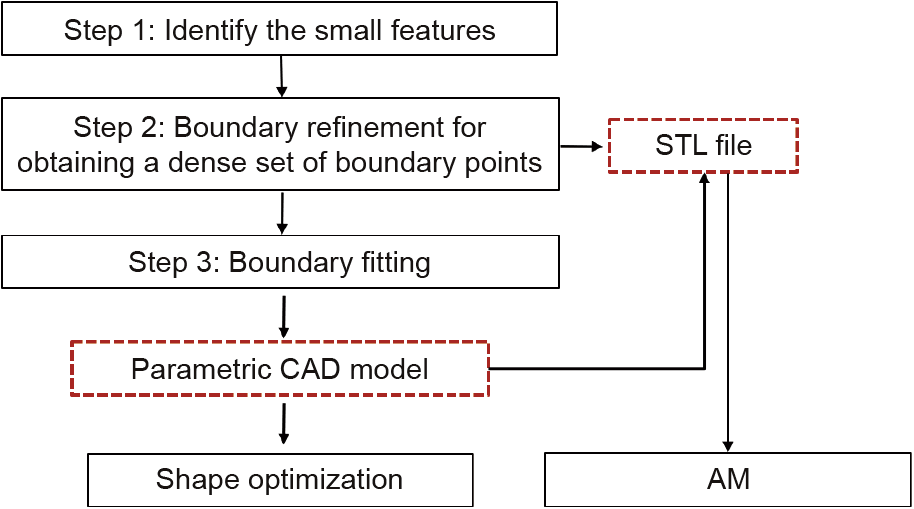
Fig. 1. Flowchart of the proposed method.
This paper is organized as follows: Section 2 provides an overview of density-based topology optimization; in Sections 3 and 4, the process of the new method is presented, using the cantilever beam as an example; and in Section 5, two more numerical examples are shown to illustrate the robustness of the proposed method.
《2. Density-based topology optimization》
2. Density-based topology optimization
《2.1 Overview》
2.1 Overview
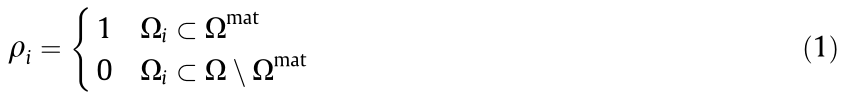
Topology optimization attempts to answer the question of what the best distribution of material within a prescribed domain is; it can be traced back to the homogenization method for topology optimization that was proposed by Bendsøe and Kikuchi [37]. On this basis, Bendsøe [38] and Zhou and Rozvany [3] proposed the solid isotropic material with penalization (SIMP) method, which is regarded as a milestone in the development of topology optimization. The basic idea of the SIMP method is to discretize the design domain by means of a finite element mesh, and to optimize the element density,  , which is either 1 or 0 depending on whether the element is filled with material or void. Fig. 2 shows the topology of a structure, in which the black elements (=1) represent the material and the white elements ( =0) represent the void. The mathematical formulation of the element density can be written as follows:
《Fig. 2》

Fig. 2. Illustration of the density-based topology optimization.
Where Ωi is the domain of the ith element, Ω represents the design domain, and Ωmat represents the structural topology. In order to solve this discrete optimization problem, the elastic modulus Ei of the ith element is defined as follows:

Where p is the penalization power. For p =1 this problem corresponds to the classical variable thickness sheet optimization”that was first studied by Cheng and Olhoff [39]. Studies showed that many grey density elements with 0 < < 1, which have no physical meaning, are obtained. Thus,  > 1 is used in order to yield distinctive " 0– 1”designs. It should be noted that choosing a p that is too low or too high causes either too many grey density elements or too-rapid convergence to local minima; therefore, a proper value of p is needed. Many numerical examples show that p=3 ensures good convergence to a solution that is close to 0–1.
This paper considers the minimal compliance problem, which is widely used for testing various new methods in the literature. The mathematical formulation can be written in the finite element form as follows:
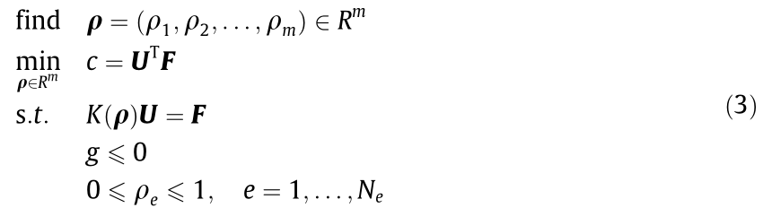
where  is the design variable vector, which is composed of the element-wise element density
  ; m is the number of design variables;
  represents the set of m real numbers; c is the structural compliance, and is used as the objective function; K is the global stiffness matrix; U is the displacement vector; and F is the external load vector. The variable g represents the volume constraint, which is measured as follows:
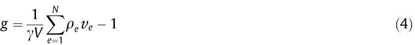
where ρe is the element-wise element density, ve represents the element volume, γ is the volume fraction, and V is the total volume of the design domain. In this paper, γ =0.3 is used, and the material properties of the structure are isotropic, with a Young’s modulus of E0 = 1 MPa and a Poisson’s ratio of v =0.3. The gradient-based iterative method—method of moving asymptotes (MMA) [40] is used to solve the topology optimization model Eq. (3). Sigmund [41] has given a 99 line MATLAB code for topology optimization implementation for the compliance minimization of structures, which provides a basic flowchart for topology optimization. On the basis of the efficient 88 line MATLAB code [42], Ref. [43] provides an efficient MATLAB code to solve 3D topology optimization problems.
《2.2 Topology optimization of the cantilever beam》
2.2 Topology optimization of the cantilever beam
In this section, the topology optimization result for the can- tilever beam shown in Fig. 3 is given. The design domain measures 120 mm×40 mm, with the left side of the domain being fixed and subjected to a concentrated load acting in the negative y-axis direction on the bottom-right corner. The design domain is discretized by 30×10 four-node plane stress elements.
《Fig. 3》

Fig. 3. Illustration of the design model.
Fig. 4 depicts the topology optimization result, in which the black elements represent the structure and the white elements represent the void. It should be noted that many grey density elements, which have an element density lower than 1 and greater than 0, exist in the topology optimization result, and it is unclear how to manufacture these grey elements. Thus, it is very important to find methods to interpret design results with grey elements into clear 0–1 and readable results for 3D printing.
《Fig. 4》
Fig. 4. The topology optimization result.
Liu and Tovar [43] have tried to apply the density threshold or density contour method to transform topology optimization results into a clear 0–1 result, and have written a MATLAB function Top3dSTL_v3 to write an STL file of the 0–1 result. Fig. 5 shows theSTL models that are obtained using these two methods,respectively. This figure shows that the obtained results contain unwelcome thin parts (point-point connections) or isolated islands. The purpose of this paper is to solve these two problems.
《3. Transformation of topology optimization results into STL》
3. Transformation of topology optimization results into STL
In this section, a new post-processing procedure with two main steps is proposed to obtain clear 0–1 topology optimization results without point-point connections and isolated islands. Next, MATLAB function Top3dSTL_v3 is used to write the STL file of the clear 0–1 result, which is suitable for a 3D printer.
《3.1 Extracting the skeleton of the result to identify small features》
3.1 Extracting the skeleton of the result to identify small features
As shown in Fig. 5, point-point connections or isolated islands usually appear in small structural features. Thus, in order to avoid these two phenomena, small structural features should be identified first. In our method, the skeleton and its inscribed circle radius from the topology optimization result are used to identify these small features. The steps are as follows:
《Fig. 5》
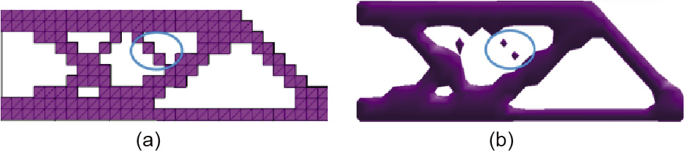
Fig. 5. The STL models obtained using Liu’s methods [43]. (a) The density threshold method (cube.stl); (b) the density contour method (iso.stl)
Step 1.1: Truncating element density and refining the mesh
Select a value of density threshold ρcutoff , and define the density of the ith element as ρi=1 when ρi> ρcutoff and as ρi=0 when ρi< ρcutoff in order to obtain an initial clear 0–1 result. Fig. 6 shows the topology optimization results for different thresholds; engineers can choose one of these according to their experience. Next, the mesh is refined in order to extract the skeleton of the result. Fig. 7 illustrates the mesh refinement, in which each mesh segment is divided into nc × nc smaller mesh segments, where nc > 0 is a positive value. It should be noted that without mesh refinement, extraction of the structural skeleton may fail.
《Fig. 6》

Fig. 6. Topology optimization results for different thresholds. (a) ρcutoff= 0:4;(b)ρcutoff=0:5; (c)ρcutoff=0.6;(d)ρcutoff=0.7
《Fig. 7》
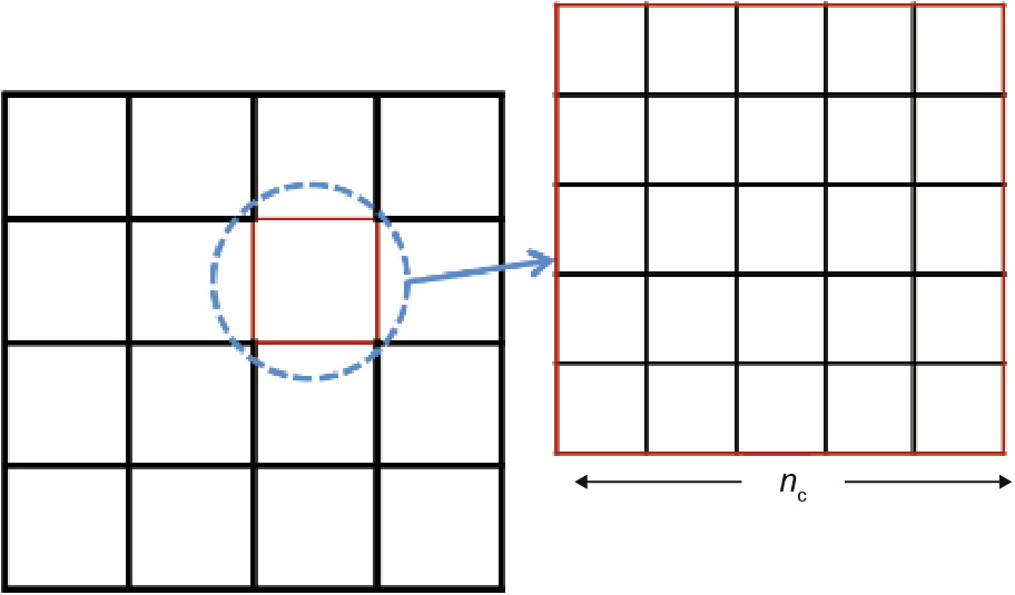
Fig. 7. Mesh refinement.
Step 1.2: Extracting the skeleton of the result and removing the burrs
Define the curve that is composed of the center of the inscribed circle which has at least two tangent points in the structural boundary, as illustrated inFig. 8. In practice, the MATLAB functions skel and spur are used to extract the skeleton and remove the burrs, respectively. The radius of the inscribed circle is defined as the feature size of the skeleton.
《Fig. 8》
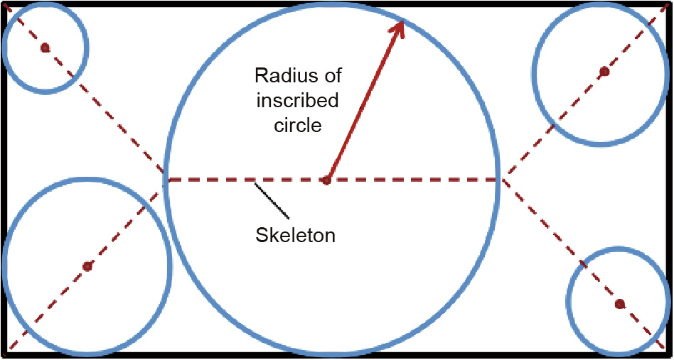
Fig. 8. Schematic illustration of the skeleton of a structure.
Step 1.3: Identifying the small features
According to the manufacturing precision of the 3D printer that is used, skeletons with a feature size (Rweak) that is lower than half of the manufacturing precision (llimit) are defined as the small features.
Fig. 9provides a flowchart for identifying the small features in a topology optimization result.
《Fig. 9》
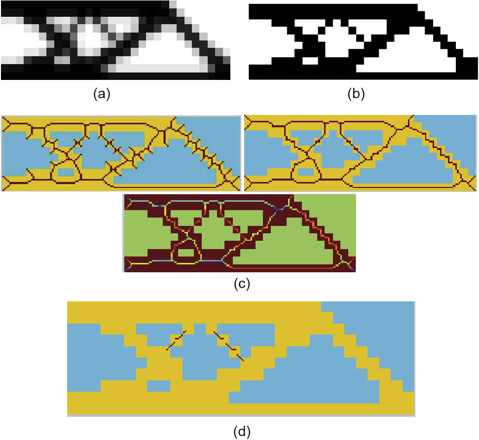
Fig. 9. A flowchart for identifying the small features in a topology optimization result. (a) Topology optimization result; (b) Step 1.1: Truncating element density and refining the mesh; (c) Step 1.2: Extracting the skeleton of the result and removing the burrs; (d) Step 1.3: Identifying the small features.
《3.2 Boundary refinement with characteristics preservation》
3.2 Boundary refinement with characteristics preservation
In order to avoid a serrated boundary with sparse nodes and isolated islands, a boundary-refinement process with characteristics preservation is performed. Fig. 10 provides a flowchart for the specific process, which includes the following steps.
《Fig. 10》
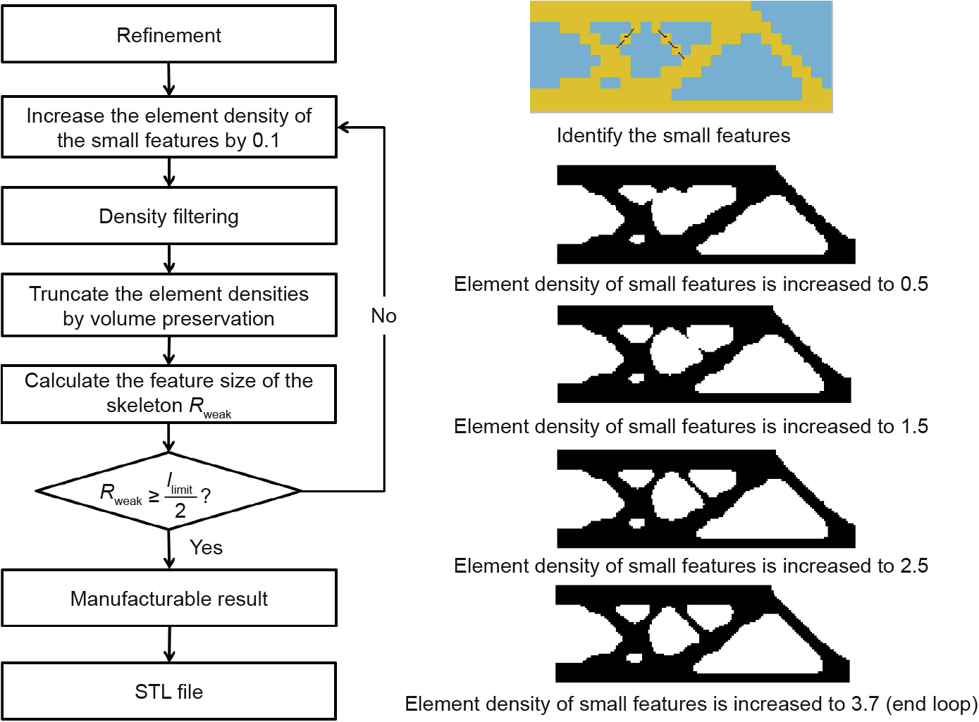
Fig. 10. Flowchart of boundary refinement with characteristics preservation
Step 2.1: Refining
Refine the mesh of the original topology optimization result. This process is similar to Step 1.1, but does not include truncating the density of the topology optimization result in advance.
Step 2.2: Handling the small features
Increase the element density of the small features by 0.1:

Step 2.3: Density filtering
Apply the density-filtering technique to avoid a serrated boundary:
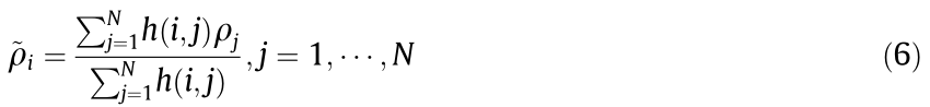
where  is the element density after density filtering;
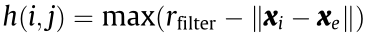 is the weight function, in which xi and xe represent the coordinates of the centers of the ith and ethelements, respectively; rfilter is the filtering radius, and rfilte= 1 in this method. After this process, a smoother boundary can be obtained
Step 2.4: Truncating the element densities by volume preservation
Truncate the element densities obtained after filtering by means of a threshold value, which is determined for volume preservation and which is calculated using the bisection method. Next, calculate the feature size of the skeleton, as described in Step 1.2, to determine whether any small features remain. If small features are still present, return to Step 2.2; if not, proceed to Step 2.5.
Step 2.5: Obtaining the STL file
Apply the density threshold or density contour to interpret the topology optimization result and obtain a clear 0–1 result. Use the MATLAB function Top3dSTL_v3 to transform the result into an STL file, as shown in Fig. 11. Compared with the results shown in Fig. 5, the results obtained by the proposed method are more suitable for manufacturing.
《Fig. 11》
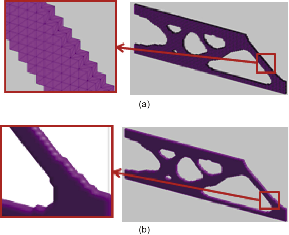
Fig. 11. The STL model obtained using the proposed method. (a) The density threshold method (cube.stl); (b) the density contour method (iso.stl).
《4. Parametric CAD model (IGES file)》
4. Parametric CAD model (IGES file)
In the previous section, we provided a flowchart for converting the topology optimization result into a clear 0–1 result with a relatively smoother boundary and denser boundary point cloud. Furthermore, an STL file, which can be directly manufactured by a 3D printer to achieve a rapid prototype, was obtained. However, as noted earlier, an STL model is not suitable for model correction.Engineers cannot modify this model to take the manufacturing constraints into consideration or reduce the stress concentration, so a parametric CAD model is preferred. Chacón et al. [35]applied a cubic uniform B-spline curve to obtain a fitting boundary for two-dimensional (2D) topology optimization results. Nevertheless, this method needs too many control points for it to be suitable for subsequent shape optimization. In this section, an adaptive B-spline fitting is proposed in order to obtain a smooth parametric CAD model with the fewest possible control points, which is suitable for shape optimization. The process is as follows:
Step 3.1: Extracting the boundary points and using a cubic uniform B-spline curve
Extract the boundary points and use a cubic uniform B-spline curve to obtain the fitting curves of the topology optimization result. Fig. 12 shows the fitted result, which has 97 control points; the red points are the boundary nodes, the black points are the control points, and the blue lines are the fitting curves. The function of the cubic uniform B-spline curve is expressed as s u .
《Fig. 12》
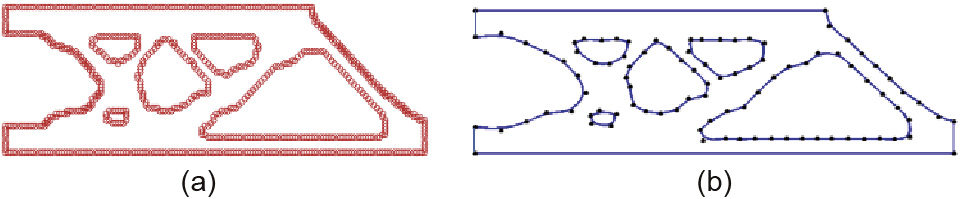
Fig. 12. Cubic uniform B-spline curve-fitting result. (a) Boundary nodes; (b) fitting result (97 control points).
Step 3.2: Reducing the number of control points
In order to reduce the number of control points, we propose a strategy to determine the locations of the nodes used in the nonuniform B-spline curve fitting. The basic idea is to reduce the number of control points in the straight lines and para-curves, which allows the curvature k(ui) and the derivative of curvature vi (ui ) of the uniform B-spline curve to be calculated as follows:
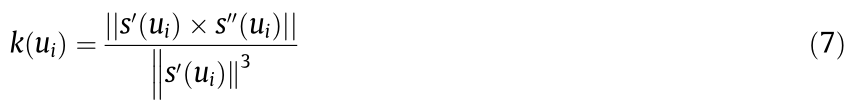

where  denotes the 2-norm; and s'(ui) and s''(ui) represent the first and second derivative of s(u), respectively. Fig. 13(a) denotesa cubic uniform B-spline curve that is used for boundary fitting and Fig. 13(b) shows the curvature and the derivative of curvature of one of the uniform B-spline curves.
《Fig. 13》

Fig. 13. Illustration of the adaptive B-spline fitting. (a) A cubic uniform B-spline curve is used for boundary fitting; (b) the curvature and the derivative of curvature of the uniform B-spline curve; (c) the adaptive B-spline fitting (43 control points).
Step 3.3: Obtaining a standard IGES file
According to geometry theory, a large s ' (ui) value represents a turning of the curve and a large s ''(ui) value represents the adjacent point between a turning and a straight line. In this paper, a threshold value, kthreshold , is chosen. Points with s ''(ui) > kthreshold are set as the nodes (i.e., the green points shown in Fig. 13(a)) and the middle point between two nodes is set as the control point (i.e., the black points shown in Fig. 13(a)). Non-uniform fitting curves can then be obtained.
The adaptive B-spline fitting is shown in Fig. 13(c); only 43 con- trol points are used, of which the red points are boundary nodes,the black points are the control points, and the blue lines are the fitting curves.
By using the MATLAB function igesout, it is possible to obtain a standard IGES file from the B-spline curve. Fig. 14(a) and (b) show the parametric model of the topology optimization result in CAD software and in computer-aided engineering (CAE) software, respectively. Fig. 14(c) shows a specimen that was fabricated using the fused deposition modeling (FDM) technique.
《Fig. 14》

Fig. 14. Parametric model of the topology optimization result. (a) Rhinos (CAD) software; (b) ANSYS (CAE) software; (c) specimen fabricated using FDM.
《5. Numerical examples》
5. Numerical examples
In this section, two numerical examples are provided to demonstrate the efficiency and robustness of the proposed method. Furthermore, a shape optimization is performed to reduce the stress concentration in the second example.
《5.1 Heat conduction problem》
5.1 Heat conduction problem
In the first example, we consider a heat conduction problem.The design domain is a square plate with the dimensions 50 mm×50 mm, as shown in Fig. 15(a). All the sides are set as insulating boundaries, and the temperature of the red point is set as T = 0.The center of the design domain has a heat source Q. The topology optimization result is shown in Fig. 15(b), which is a tree-like topology.
《Fig. 15》
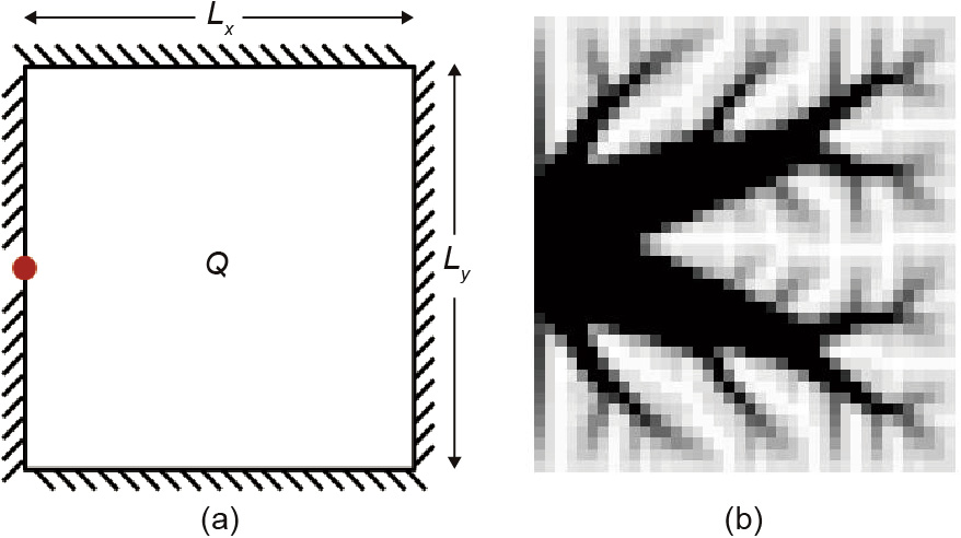
Fig. 15. (a) The design domain of the heat conduction problem; (b) the topology optimization result.
Next, we apply the proposed method to this topology optimization result in order to obtain a CAD model. Following the procedures described above, we first identify the small features and then refine the boundaries while preserving the characteristics (Steps 1 and 2). Fig. 16 shows the results after each sub-step. The parameters pcutoff=0.2 and nc =8 are used in these two steps.
《Fig. 16》

Fig. 16. Results of the heat conduction problem obtained after Steps 1 and 2. (a) Steps 1.1 and 1.2; (b) Step 1.3; (c) Step 2.
Two parametric CAD models are then obtained by using uniform fitting and adaptive fitting, respectively. For the uniform fitting result, 439 control points are needed to obtain a smooth result, while only 201 control points are needed for the adaptive fitting. Fig. 17 depicts the CAD models that were obtained using these two methods, and the resulting specimens that were fabricated using FDM. The red points are the boundary nodes, the green points are the control points, and the blue lines are the fitting curves.
《Fig. 17》

Fig. 17. CAD models of the fitting results and corresponding products fabricated using FDM.(a)Uniform fitting result; (b) adaptive fitting result.
《5.2 L-shape beamFig.》
5.2 L-shape beamFig.
In this section, the example of an L-shape beam is used to validate the efficiency of the proposed method, and a shape optimization is performed to reduce the stress concentration in the corner. The design domain and its topology optimization result are shown in Fig. 18.
《Fig. 18》
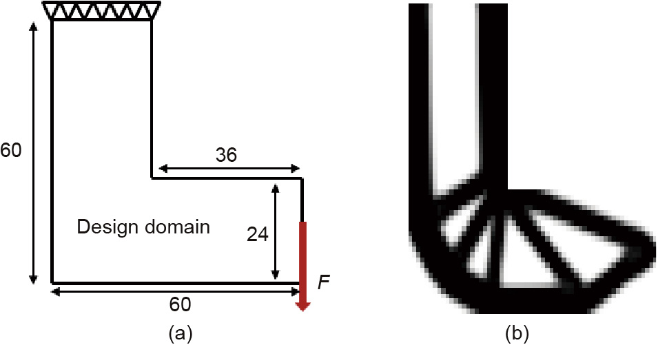
Fig. 18. (a) Design domain of an L-shape beam (unit: mm); (b) the topology optimization result.
The same process used with the first example is used here. Fig. 19 shows the results after Steps 1 and 2. The parameters pcutoff= 0.5 and nc =8 are used in this example.
《Fig. 19》
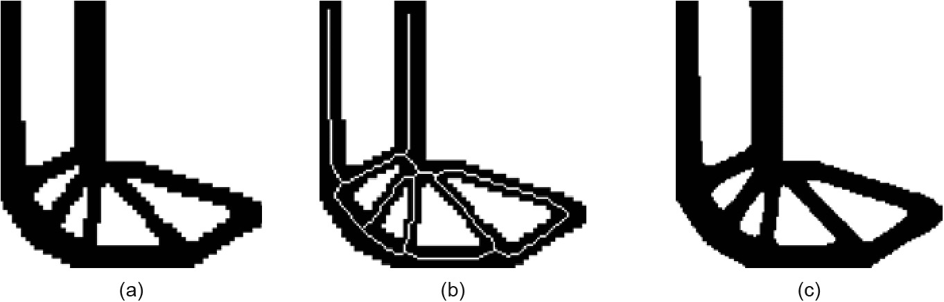
Fig. 19. Results of the L-shape beam obtained after Steps 1 and 2. (a) Steps 1.1 and 1.2; (b) Step 1.3; (c) Step
Two parametric CAD models are then obtained by using uniform fitting and adaptive fitting, respectively. For the uniform fitting result, 113 control points are needed to obtain a smooth result, while only 57 control points are needed for the adaptive fitting. Using the new method proposed in this paper, a parametric CAD model is obtained, as shown in Fig. 20. The red points are the boundary nodes, the black points are the control points, and the blue lines are the fitting curves.
《Fig. 20》
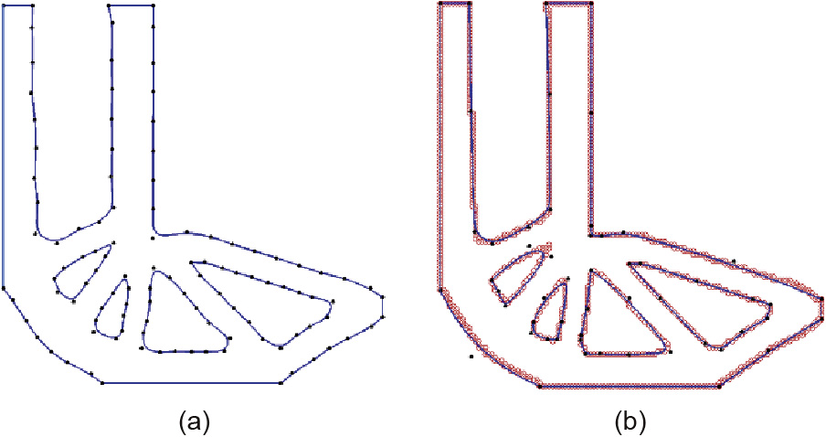
Fig. 20. CAD models of the fitting results. (a) Uniform fitting result; (b) adaptive fitting result.
Using the MATLAB function igesout, a standard IGES file based on the adaptive fitting result is obtained, and a finite element model, as shown in Fig. 21, is established. All freedoms on the top side are constrained, and a force of P =100 N is applied on the middle of the right side (the red arrow in Fig. 21). The finite element size is 1, the elastic modulus of the material is 236 MPa, and the Poisson’s ratio is 0.3.
《Fig. 21》
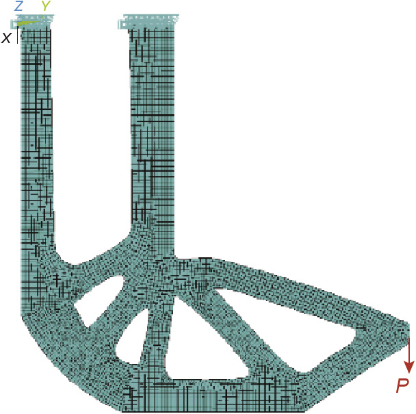
Fig. 21. Finite element model of the parametric model.
In order to reduce the stress concentration in the corner, a shape optimization problem is performed, as formulated below:
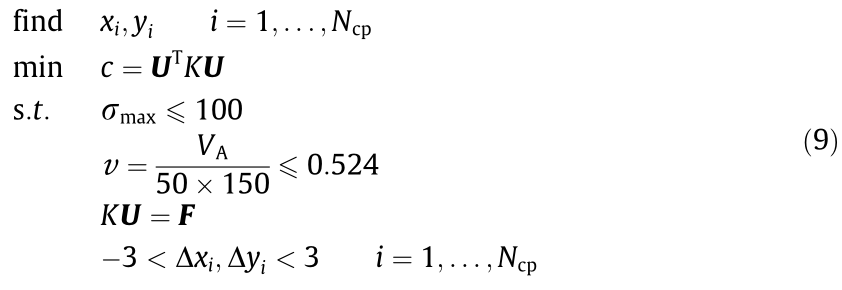
where  is the maximum stress of the structure under the force P; xi, yi are the coordinates of the ith control point, and are set as design variables; Ncp is the number of control points; and VA is the volume of the optimized structure. Other symbols have the same meanings as Eq. (3). Volume constraint and stress constraint are considered in this paper. The multi-island genetic algorithm (MIGA) is used to solve this problem, and the optimized result is shown in Fig. 22(b).
《Fig. 22》
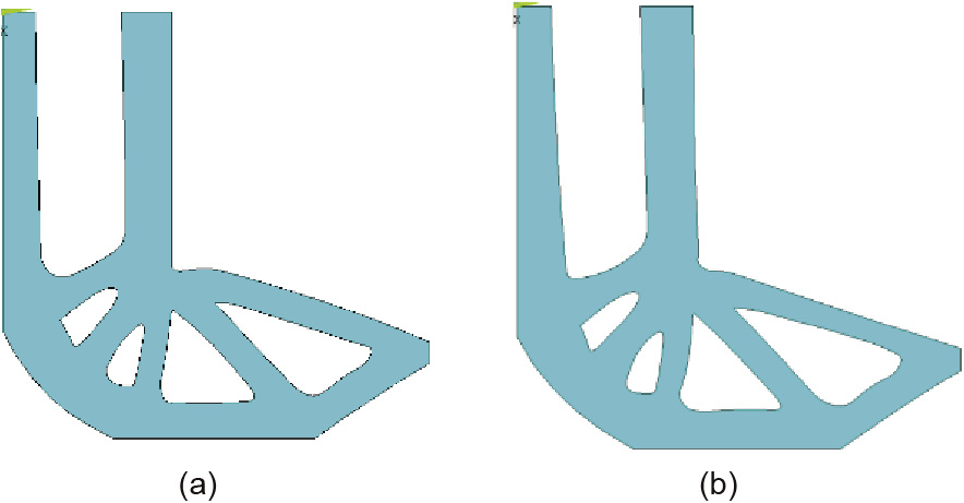
Fig. 22. Optimized results before and after shape optimization. (a) Result before shape optimization; (b) result after shape optimization.
The finite element method is used to analyze these two results, and the von Mises stress nephograms are shown in Fig. 23. A comparison of these two results reveals that the maximum von Mises stress is reduced from 110 MPa to 77.3 MPa after the shape optimization.
《Fig. 23》

Fig. 23. Von Mises stress nephograms for the two results. (a) Von Mises stress nephogram before shape optimization; (b) von Mises stress nephogram after shape optimization.
《6. Conclusions》
6. Conclusions
This paper presents an automatic method for converting a topology optimization result into an STL file that is suitable for AM. In the proposed method, the skeleton of the topology results is extracted to ensure shape preservation, and a filtering method is used to ensure characteristics preservation. After this process, a relatively smoother boundary of the topology optimization result with a denser boundary point cloud is obtained. An adaptive B- spline fitting is proposed in the obtained input to obtain a smooth, parametric CAD model with fewer control points, which is suitable for shape optimization to improve the performance of the result. This approach to interpreting topology optimization results reduces the time that is required to utilize the results and helps to standardize the interpretation process.
《Acknowledgements》
Acknowledgements
The authors gratefully acknowledge financial support for this work from the National Natural Science Foundation of China (11332004, 11372073, and 11402046), the 111 Project (B14013),and the Fundamental Research Funds for the Central Universities (DUT15ZD101).
《Compliance with ethics guidelines》
Compliance with ethics guidelines
Shutian Liu, Quhao Li, Junhuan Liu, Wenjiong Chen, and Yongcun Zhang declare that they have no conflict of interest or financial conflicts to disclose.


 京公网安备 11010502051620号


