
《1. Introduction》
1. Introduction
Autonomous robots can acquire information on the environment and assist humans in various circumstances and applications, such as rescuing humans from danger, providing service within urban or home environments, and guiding or otherwise aiding people in need [1–6]. Despite the dramatic development of relative technologies and algorithms, major challenges remain. The complexity and variability of the unknown environment make it difficult for human operators to provide prior information to a robot [7]. Thus, it is of great significance to equip a robot with the capabilities of autonomous exploration and mapping, including incremental map construction, localization, path planning, motion control, navigation, and so on, without direct human intervention.
Heuristic and reactive exploration approaches have been studied in the literature. In Ref. [8], Yamauchi proposes a frontier-based heuristic exploration algorithm. In Ref. [9], based on the angular uncertainty of sonar sensor, a heuristic exploration strategy is proposed that uses a sonar sensor array for perception and mapping. In Ref. [10], a local map-based frontier graph search exploration method is developed, and the environment is represented by a tree structure, making it efficient to determine the next target position even within a large environment. In Ref. [11], Keidar and Kaminka describe a morphological frontier detection method using light detection and ranging (LIDAR) data to accelerate the map frontier point detection process. In Ref. [12], a reactive exploration strategy is proposed that uses current velocity and bearing for rapid frontier selection.
The simulation-based autonomous exploration strategy has been attracting increasing research effort, since it can assist in measuring information and generating the goal pose based on a current robot’s status during exploration. In Ref. [13], Carrillo et al. propose a utility function with Shannon and Rényi entropy in order to measure the robot’s actions for exploration. In Ref. [14], Lauri and Ritala present a forward simulation algorithm, and formulate the exploration to a partially observable Markov decision process (POMDP). In Ref. [1], with partially known environment information, a red/green/blue-depth (RGB-D) sensor is used for loop closure detection in an autonomous mapping and exploration process. In Ref. [15], Bai et al. propose a Gaussian process regression-based exploration strategy, and predict mutual information with robot motion samples. In Ref. [16], the autonomous exploration problem is formulated as a partial differential equation; the information is described as a scalar field from the prior known area to the unknown area.
In existing exploration methods, range sensors are mostly used and two-dimensional (2D) grid maps are generated. However, a 2D grid map only contains planar geometric information, and is often insufficient for human perception [17–19]. RGB-D sensors directly provide both color and depth information, and can help to generate a three-dimensional (3D) point cloud map. RGB-D sensor-based simultaneous localization and mapping (SLAM) systems were first proposed independently by Henry et al. [20] and Engelhard et al. [21]. Image features were used to find matches among each frame, and an iterative closest point (ICP) algorithm was applied to estimate the point cloud transformations in the RGB-D SLAM systems. In Ref. [22], Klein and Murray present the parallel tracking and mapping (PTAM) framework and implement tracking and mapping in dual parallel threads. Labbé and Michaud [23] propose the real-time appearance-based mapping (RTABMAP) algorithm, in which loop closure detection thread and a memory management method are added. Online incremental mapping and loop closure detection can be attained, and the mapping efficiency and accuracy can remain consistent over time.
The field of view (FoV) of existing RGB-D sensors is limited [24]. To obtain a greater scope of environment information, multiple RGB-D sensors can be used together. Dual RGB-D sensors have been utilized in visual SLAM for robust pose tracking and mapping [25], and an RGB-D sensor has been fused with an inertial measurement unit (IMU) for indoor wide-range environment mapping [26]. In Ref. [27], Munaro et al. present an RGB-D sensor network, in which multiple RGB-D sensors are deployed in an indoor environment for human tracking. In Ref. [28], multiple RGB-D sensors with non-overlapping FoVs are employed for line detection and tracking, thus providing a 3D surrounding view and morphological information on the environment.
In our previous work, we developed RGB-D-based localization and motion planning and control methods [24], and realized RGB-D-based exploration [17]. Nevertheless, the robustness and efficiency of the exploration process was limited due to the small FoV of the RGB-D sensor. In this work, we used dual RGB-D sensors for the mobile robot. The deployment of dual RGB-D sensors provided a larger FoV, but also introduced technical challenges in interference, data synchronization, and processing. With the synchronized data from the dual RGB-D sensors, location points were generated and a 3D point cloud map and 2D grid map were incrementally constructed. An autonomous exploration strategy was established by combining partial map simulation with global frontier search methods. In this way, the local optimum can be avoided and the exploration efficacy can be ensured. The experimental results demonstrated the high robustness and efficiency of the developed system and methods.
This paper is organized as follows: Section 2 presents the 3D and 2D mapping method with dual RGB-D sensors, and Section 3 describes the autonomous exploration algorithm in detail. Section 4 describes the mobile robot system that validates the proposed mapping and exploration method. Section 5 presents the experiments and results. Finally, Section 6 concludes the paper.
《2. Mapping with dual RGB-D sensors》
2. Mapping with dual RGB-D sensors
With the information provided by dual RGB-D sensors, a 3D point cloud map can be constructed in real time. This process includes location point creation, mapping, and loop closure detection.
《2.1. Location point generation》
2.1. Location point generation
Fig. 1 presents the process of creating location points. In order to construct a 3D point cloud map, the sensor data must be processed; this includes the RGB images and depth images from the dual RGB-D sensors, and the wheel odometry data from the mobile chassis. The data should then be synchronized. The pose between the dual RGB-D sensors is known, as it can be determined by calibration after system assembly.
《Fig. 1》
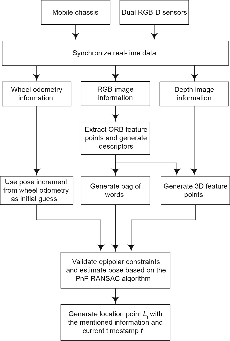
Fig. 1. The process of location points creation.
Past information is not included in the current frame of the information queue, including RGB images, depth images from the dual RGB-D sensors, and the wheel odometry information. Fig. 2 depicts the synchronization implemented with the robot operating system (ROS) message filter method.
《Fig. 2》

Fig. 2. Sensor data synchronization.
The synchronized sensor data are processed to create location points. Dual RGB-D color and depth data are simultaneously combined into an integrated data structure that comprises the current sensor data, which can be used for the location point creation process. The oriented fast and rotated brief (ORB) feature points and corresponding descriptors are obtained from the RGB images. The 3D feature points in the robot frame are integrated with the 2D feature points and with corresponding depth data from the depth images, as the pose between the dual RGB-D cameras is known. The fundamental matrix based on the epipolar constraint is calculated in order to determine the inliers, using matched 3D feature points from the last frame and the current frame. With enough inliers, data from the wheel odometry is extracted to provide an initial guess of the transformation between the last frame and the current frame.
The transformation between the frames is estimated by the random sample consensus (RANSAC) algorithm based on the perspective–n–points (PnP) model, using matched 3D feature points. The bag of words (BoW) of a frame is created by corresponding ORB descriptors, and the environment vocabulary is incrementally constructed with the BoW online, rather than pre-training in the target environment, as doing so is more suitable for autonomous exploration tasks. The location point, Lt, is created with the above information and the current timestamp, t, and the edge between the last and current location point is initialized, with its weight set to zero.
Depth errors and feature mismatch errors may exist in an unknown environment, especially in a place with few features and varying illumination. A sudden change in RGB-D localization may occur, which can detrimentally impact the real-time motion control of the mobile robot. Furthermore, although wheel odometry changes smoothly, it contains accumulated error. However, the RGB-D localization and wheel odometry can be fused by means of an extended Kalman filter in order to achieve robust localization.
《2.2. Point cloud mapping and loop closure detection》
2.2. Point cloud mapping and loop closure detection
The mapping and the loop closure detection process are tightly coupled using graph optimization and memory management methods to ensure stability and real-time performance. The similarity and pose of the location points are optimized in the treebased network optimizer (TORO) framework [29] to ensure global consistency.
The location points are stored in the working memory (WM) or long-term memory (LTM), as determined by the similarity, as shown in Fig. 3. The location points in the WM are used for realtime loop closure detection, while other location points are stored in the LTM as candidates. The candidates will either be retrieved to the WM or deleted, according to their similarity and storage time in the LTM.
《Fig. 3》

Fig. 3. The process of mapping and loop closure detection.
First,  is set as a new vertex of the graph and the similarity of and the nearest M location points is calculated by their BoWs, as shown in Eq.(1), where
  represents the matched BoW number between the BoW of and a BoW from one of the nearest N location points,
  .
.  and
and  are the BoW numbers of and , respectively. The similarity of and is marked as λ. When λ is greater than the threshold, ε, is merged into and is loaded into WM.

The conditional probabilities of the loop closure among and other location points on the graph are updated with λ. The weight of the graph edges among and the other location points are corrected by TORO, including the location points in the WM and LTM. The transformations among and the location points in the WM are calculated by the ICP algorithm, with an initial guess from the wheel odometry. Loop closure is established if the variation is smaller than the given threshold. With the estimated current transformation, the weights of the edges are updated and the poses of other location points are corrected to ensure the global consistency of the pose from each location point. The location point in the WM with the lowest weight and longest residence time will be transferred to the LTM, and the location point in the LTM with the greatest weight will be retrieved to the WM. The global 3D point cloud map is updated with the corrected information from the graph.
Fig. 4 shows the 3D point cloud segmentation and 2D grid map construction process with dual RGB-D sensors. The point cloud map is voxelized and down-sampled with the voxel filter in the Point Cloud Library (the voxel size is set as 0.05 m). A point set is selected and its normal vector is estimated by the k nearest neighbor algorithm. The point set size k is set as 10, which reconciles the computing efficiency with the precision. The normal vector is estimated as shown in Eq. (2).

《Fig. 4》
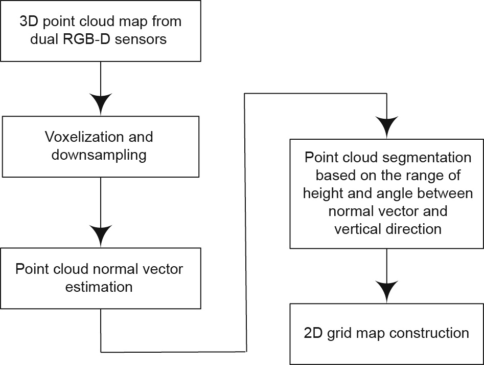
Fig. 4. The process of 3D point cloud segmentation and 2D grid map construction.
Here,  is the coordinate of each point and
  is the center coordinate of the corresponding point set. C is the covariance matrix, and
  and
and  are the eigenvector and eigenvalue of C, respectively. The eigenvector with the biggest eigenvalue,
  is selected as the normal vector of the point set,
  [30]. The point sets in the point cloud can be determined and segmented with the above information. If the point set has a normal vector that deviates from the vertical direction by more than a given threshold, it is set as an obstacle. Otherwise, it is possible to move to the next step. The point set is then processed with the Euclidean clustering extraction method. If the height of its center is greater than a given threshold, the point set will be set as an obstacle. Otherwise, it is taken as free space. The grid map is constructed with the (x, y) coordinates from the obstacle portion of the point cloud.
A robot may pass by a region with few visual features or with features that are similar to the surroundings, which leads to the failure of loop closure detection [31]. In such circumstances, the mobile robot can execute autonomous motion in the exploration process; this changes the FoV of the dual RGB-D sensors in order to obtain more environment information.
《3. Autonomous exploration》
3. Autonomous exploration
The real-time updated 2D grid map and localization are set as prior information for the autonomous exploration. The updated map and odometry information are used for the next goal pose generation, so as to expand the map and further explore the environment.
《3.1. Autonomous exploration based on the POMDP model》
3.1. Autonomous exploration based on the POMDP model
Assuming that the environment is partially known and contains stochastic information, the mobile robot exploration process can be described by a POMDP model  .
.
•  represents the decision epoch of the goal generation in the exploration task.
•  represents the state space of the exploration task, including the mobile robot state
 and the map state
  and
and are both observable. (The errors from applying a given motion to the robot and from applying the localization data are not considered, so
 is completely observable and is partially observable.)
•  represents the feasible motion according to the robot motion constraint.
•  represents the observation space.
•  represents the state transfer model, which consists of
  and
and  describes a state transfer
  from the current mobile robot state
  and motion
 to the next state,
 .
. represents the scope of occupancy grid probabilities.
  is independent of
  , which means that
 for any
  .
.
•  represents the observation model, as shown in Fig. 5. According to the current mobile robot pose and the 2D grid map, an observation value of the current state is taken by ray tracing the model.
《Fig. 5》

Fig. 5. The exploration process based on the POMDP model.
•  represents the reward function constructed by the state, observation, and action, as measured by the belief state value. Mutual information function is chosen as the form of the reward function.
Based on the 2D grid map and the robot pose, a series of mobile robot motions are generated for trajectory simulation, from which the current goal pose is selected. The motions are evaluated by the reward function, with the target being to maximize the reward function in the corresponding decision epoch. In the POMDP model-based exploration process, the reward function is defined as the mutual information function, as in Eq. (3).  represents the reward function value in decision epoch k, which is determined by the states of N particles. Particles are simulated from the belief state
  and
and  , with the robot state
  ; and with the observation
  of the map state
  .
.

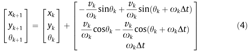
The first term of Eq. (3) is the expected information gain of the mobile robot state. Considering that the experimental environment is a flat terrain on which the given motion can be executed correctly, we assume that there is no noise in the mobile robot motion model 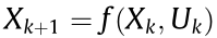 [32], as shown in Eq. (4). This assumption aligns with the decision to choose the particle state with the maximum likelihood value
  as the expected result. Therefore, the mutual information gain described by the robot state and observation is set as 0.
The second term of Eq. (4) is the expected information gain of the map state, which is represented by the mutual information gain of the map state and the observation value. The integral is implemented by summing up the entropy of the selected grids during the simulation. The probability range of the grid is [0,1] : 0 for the free state and 1 for the occupied state. The entropy of the binary random variable is defined in Eq. (5).

The entropy summing scope is set based on the ray-tracing observation model of the sensor. The model is described as follows: Define a sector with  as the origin, the maximum observation range r as the radius, and the observation angle θ as the center angle. Select the probability value of the grids in the ray-tracing beam direction of the sector and calculate the corresponding entropy value. For grids with an unknown probability (which means that the grid is in the unknown environment), set the entropy value as 1.
《3.2. Partial map simulation and global frontier search》
3.2. Partial map simulation and global frontier search
The mobile robot autonomous exploration process is described by the POMDP model, in which the goal pose of each epoch is generated by the combined strategies of partial map simulation and global frontier search, as shown in Fig. 6. A goal pose Xg and its reward function value Rg is generated by the partial map simulation process with the current 2D grid map and robot pose. This process is listed as Procedure 1, and contains particle sampling, weight calculation, and resampling. The parameters include the iteration number I, particle number N, sampling number  , sample distribution kernel function
  ; ray-tracing model
  ; simulation stage H; resampling lower bound
  ; and discount factor
  .
.
《Fig. 6》

Fig. 6. Diagram of the exploration strategy.
The partial map simulation process based on the POMDP model is presented in Procedure 1. First, the algorithm iterates over  and simulates particles over
  . Based on the iteration number, a kernel function
  is chosen for particle sampling, generating the motion series
  . For uniformity of the initial sampling and a better solution for subsequent sampling,
  is set as a uniform distribution and
  is set as a normal distribution with the mean from by initial sampling . The range of the uniform distribution
  and the covariance matrix of the normal distribution
  are set based on the velocity range of the mobile chassis. Current particle poses are updated based on the mobile robot motion model and the generated motions. The map observation is updated from the ray-tracing model and given an observation range, and the reward function value of each particle is also updated. The sampling number
  is an increasing linear sequence of
  , and is a faster way to converge to the optimal solution of the probability meaning. The weights of the particles are updated after the simulation stage has occurred H times. The prior and posterior information are evaluated with observation
  , based on ray-tracing model
  and the inverse sensor model. In practical applications, the reward function is calculated using prior and posterior information. The log odds of the prior and posterior probability are calculated, with random value
  as the noise of the inverse sensor model. The discount factor
  indicates the relationship between the simulated information and the current information. For example,
  means that further simulated information takes on more weight. If the weights of the particles are overly dispersed,
  ; then the particles should be resampled and new particle poses and map observations should be generated. The goal pose and corresponding reward function value are simulated from the motion series with maximum weight.
The optimization time and simulation range must be limited. An optimal solution of the probability meaning can be reached for the partial map simulation process by means of the Monte Carlo method over a limited simulation range. The mobile robot may continue to pace around, or may get stuck when entering the region with the local information optimum. Thus, a global frontier search strategy is introduced in order to avoid a local optimum.


Frontiers between the known region (which is constructed by the exploration process) and the unknown region are detected by means of a global frontier search strategy based on a breadth-first search algorithm. The nearest connected frontier point to the current mobile robot pose is selected, and the connected point is defined as a point with eight existing grids around it. The exploration time and region cannot be ensured, as the observable unknown environment near frontier points cannot be determined by such a heuristic search strategy. The global frontier search strategy can avoid a local optimum using the current known map. Information on the unknown environment can be measured by means of the partial map simulation strategy, thus ensuring new information is obtained within each exploration epoch. The combined strategy is shown in Fig. 6. The goal pose  and its reward function value
  are generated by the partial map simulation. If
  ; the goal pose can be sent to the motion control process. Otherwise, the global frontier search strategy is triggered for a new goal pose. The new exploration process begins when the mobile robot arrives at the goal pose within a given time; alternatively, the current exploration and the motion control process will be suspended if the time exceeds the limit.
The lower bounds of the reward, iteration number, and particle number mainly affect the efficiency and robustness of the exploration process. The lower bound ensures the efficiency of the partial map simulation, and a local optimum can be avoided with a global frontier search. More information can be obtained when using increased iterations and particles, but the efficiency may decrease with the resulting heavier computation.
《4. System implementation》
4. System implementation
《4.1. System implementation with dual RGB-D sensors》
4.1. System implementation with dual RGB-D sensors
A mobile robot system was constructed to validate the proposed autonomous exploration and mapping method. The system consisted of a Yujin Kobuki mobile chassis, dual Kinect RGB-D sensors, and an HP Envy 15-j105tx mobile computing unit. The environment color and depth data obtained by the Kinect were used in the method. The resolution of the RGB and depth images was 640×480 pixels, with a frequency of 30 Hz. The FoV was 57 horizontal degrees by 43° vertical degrees, and the depth range in the indoor environment was 0.5–5 m [33]. The Yujin Kobuki mobile chassis was differentially driven by the two wheels, with a diameter of 0.46 m, a maximal linear speed of 70 cm·s-1 , and an angular speed of 180·s-1 . The frequency of the wheel odometry had a maximum of 50 Hz. The mobile computing unit was equipped with a CPU i7 4702 M and 8 GB RAM. ROS Indigo, OpenNI RGB-D driver, the Point Cloud Library, and OpenCV were also installed on the mobile computing platform.
Kinect obtains depth data by means of structured light measurement, mainly by projecting an infrared speckle to the measured object and capturing the depth information through the complementary metal-oxide semiconductor (CMOS) infrared sensor. An interference problem occurs in situations when multiple Kinect FoVs overlap [34]. To avoid structured light interference among the sensors and to expand the FoV of the system, dual Kinect RGBD sensors were installed, as shown in Fig. 7; their pose relative to the mobile chassis is shown in Eq. (6).  are the translation and ZYX Euler angles of the Kinect frame relative to the mobile chassis. The transformation among the dual Kinect RGB-D sensors and the mobile chassis is given by Eq. (6).

《Fig. 7》
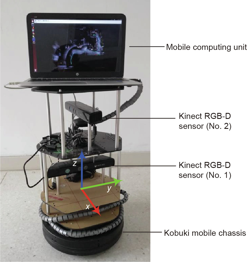
Fig. 7. The mobile robot hardware platform.
《4.2. System workflow》
4.2. System workflow
Fig. 8 shows the mobile robot autonomous exploration and mapping workflow.
《Fig. 8》

Fig. 8. The workflow of the mobile robot for autonomous exploration.
(1) Mapping and localization. According to the environment RGB-D information that was obtained by the dual Kinect RGB-D sensors and the wheel odometry from the mobile chassis, the RTABMAP algorithm was adopted to estimate localization information. The pose was fused with the RGB-D localization and wheel odometry based on an extended Kalman filter (EKF, integrated in the ROS robot_pose_ekf package), and a 3D point cloud map was constructed. A 2D grid map was generated from the 3D point cloud for autonomous exploration and motion control.
(2) Combined strategy of partial map simulation and global frontier search. Based on the forward simulation algorithm, the goal pose  of the exploration process was generated using the 2D grid map and the current pose
  ,with the simulation strategy using partial information from the grid map, and the search strategy using global frontier points from the grid map.
(3) Dynamic window motion control based on motion constraints. According to the robot’s current pose  ; a 2D grid map
  ; and a goal pose
  from the exploration strategy, the robot’s motion control command was generated. To ensure the stability of the mapping process, cost function was added with the motion constraint, based on a dynamic window control algorithm [35].
In the exploration algorithm, the distance between an available goal and the current position was set to be between 0.5 and 10 m, the maximum speed of the robot was 0.5 m·s-1 , and the cycle time was below 1.0 s. During the exploration process toward the next goal, the point cloud map, grid map, and pose were updated to provide environment information. The point cloud and grid map update rate was 1 Hz, and the pose update rate could be increased up to 20 Hz. Thus, these parameters were able to meet the demands of the exploration process.
《5. Experiments and results》
5. Experiments and results
《5.1. Experimental settings》
5.1. Experimental settings
The autonomous exploration and mapping environment settings are shown in Fig. 9(a). The mobile robot set off in the starting region and executed the autonomous exploration and mapping task. The task was finished when the robot arrived at the target region. Eight kinds of indoor scenes were tested, as shown in the figure. Scene (i) was a rectangular area with obstacles on three sides and only one exit. Scenes (ii–iv) were aisles with widths of 1.43 and 0.85 m, respectively ((iii), (iv) for the entrance and exit). Scenes (v) and (vii) were regions with various obstacles and aisle widths of 0.90 and 0.78 m, respectively. Scenes (vi) and (viii) were different perspectives of the open area.
《Fig. 9》

Fig. 9. The autonomous exploration and mapping experiment. (a) The experiment environment from scene (i) to (viii). The (b) constructed 3D point cloud map and (c) generated 2D grid map and mobile robot trajectory from the autonomous mapping and exploration process.
According to the mobile robot exploration process in the laboratory, the scenes were divided into two types: single connected regions and multi-branch regions. Scenes (i–iv) were single connected regions, with only one aisle connecting scene (i) to scene (iv). The mobile robot made a 90° right turn from scene (i) to scene (ii), and then a 90° right turn to scenes (iii) and (iv), in which the view of the sensors was restricted by the baffle plates and the width of the aisle. The height of the baffle plates was 1.5 m, which was greater than the vertical range of the RGB-D sensors. Scenes (v–viii) were multi-branch regions; the order in which the mobile robot explored these scenes was not unique due to the stochastic nature of the exploration algorithm. Thus, the experimental task was activated from the start region of the indoor environment and was stopped after entering the target region. The starting region was a rectangular area in the aisle, with a length of 1.18 m from the edge of the cabinet on the right side to the rear obstacle, and a width of 1.12 m. The target region was a rectangular area in scenes (vi) and (viii) bounded by the door and the wall, with a length of 2.68 m and a width of 2.44 m.
In the single connected regions, the FoV was limited, regardless of whether single or dual RGB-D sensors were deployed. In the multi-branch regions, the scene was wider, and the dual RGB-D sensors allowed more information to be detected and fed into the system. Thus, the experiment was able to demonstrate the efficacy of utilizing dual RGB-D sensors by comparing the experimental performances in the single connected and multi-branch regions.
《5.2. Results》
5.2. Results
Combining the methods of partial map simulation with a global frontier search ensures that the simulated goal pose is the optimum in the observation scope, and that a local optimum can be avoided by searching the map frontier. Thus, the exploration task was successfully accomplished.
Fig. 9(b) depicts the 3D point cloud map constructed from the mobile robot autonomous mapping and exploration experiment. This laboratory 3D point cloud map was constructed using the mobile robot odometry and the information from the dual RGB-D sensors; it includes the narrow aisles, obstacles, and open area. The constructed 3D point cloud map corresponded well with the actual indoor environment; examples of good correspondence included the rear box in scene (i), the color blocks near the wall in scene (ii), the obstacles in scenes (v) and (vii), the door in scene (vi), and the open area in scenes vi and viii. The 3D point cloud map was incrementally constructed during the autonomous exploration process, thus preserving spatial consistency with effective stitching.
Fig. 9(c) depicts the 2D grid map that was generated from the 3D point cloud map and the mobile robot trajectory. In this 2D grid map, the length of the x axis is 11.40 m, and the length of the y axis is 9.40 m. The actual dimensions of the laboratory were 11.04 m by 7.93 m. The dimensions of the starting region were 1.25 m by 1.20 m, and the dimensions of the target region were 2.80 m by 2.43 m. The size, location of obstacles, and dimensions of the 2D map matched well with the real situation.
With the combined method of partial map simulation and global frontier search, the mobile robot continuously obtained environment information during the autonomous mapping and exploration process. Furthermore, in circumstances with insufficient information, the trajectory to the destination could be recovered with sufficient information by triggering the frontier search method. If a goal pose with sufficient information could not be simulated in the current robot pose, the global frontier search strategy was triggered in order to change the view of the robot sensors for further exploratory orientation to the target region; for example, the scene might change from (iv) to (v), corresponding to (-1.7, -3.6) in Fig. 9.
Fig. 10 shows the time-region curve of the autonomous mapping and exploration process, with a comparison between the use of a single RGB-D sensor and dual RGB-D sensors. The area was measured by the generated 2D grid map. A total area of 31.0 m2 was explored over 196 s with the dual RGB-D sensors, whereas a total area of 27.6 m2 was explored over 297 s with a single RGB-D sensor. In the single connected regions, the view obtained by the autonomous mobile robot system was limited by the aisle; thus, the exploration efficiency with a single RGB-D sensor was similar to that of the system with dual RGB-D sensors. In the multi-branch regions, the exploration cost time with the dual RGB-D sensors was significantly less than with a single RGB-D sensor; furthermore, the exploration area covered with the dual RGB-D sensors was larger than the area covered with a single RGB-D sensor. The mobile robot equipped with dual RGB-D sensors obtained more environment information than when equipped with a single RGB-D sensor. In the autonomous mapping and exploration process, the map region stably increased over time, thus demonstrating the efficacy of the proposed method.
《Fig. 10》
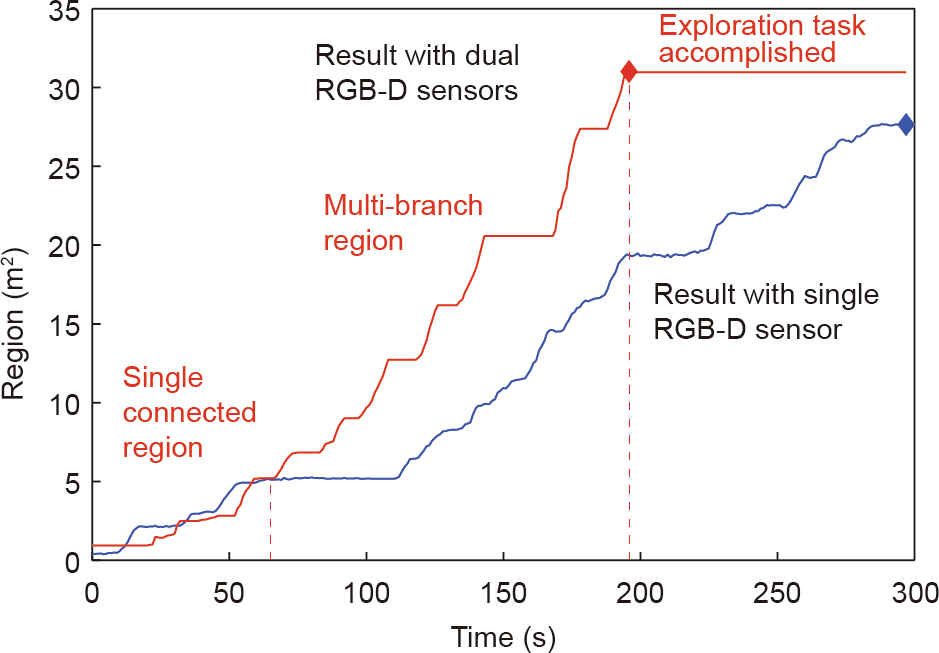
Fig. 10. The time-region curve in the autonomous mapping and exploration process comparing a single RGB-D sensor with dual RGB-D sensors.
《5.3. Discussion》
5.3. Discussion
The exploration process will be aborted if neither the partial map simulation algorithm nor the global frontier search algorithm can generate an available exploration goal. The partial map simulation algorithm may fail if no goals with sufficient information can be generated. Furthermore, the global frontier search algorithm may fail if no feasible connected frontier point can be discovered. As shown in Fig. 6, if both algorithms fail, the current exploration process is stopped. The robot can remain in place, return to the starting point, or execute orders from the human operator.
In the autonomous mapping and exploration process, the use of the dual RGB-D sensors improved the exploration efficiency. If more RGB-D sensors are deployed, the localization accuracy may be further improved, as has been observed in other applications [25]. More sensors can be integrated into the system for application-specific measurements [6]. The number and type of sensors can be determined with respect to application, computational cost, real-time capability, and accuracy requirements.
Multiple robots can collaborate in the exploration process in order to obtain more information and improve the exploration efficiency [36]. The fusion of autonomous exploration with teleoperation from human operators holds promise for overcoming possible pitfalls in robot autonomy [37].
《6. Conclusion》
6. Conclusion
In this work, we have presented a systematic approach for the autonomous exploration and mapping of an unknown environment using dual RGB-D sensors. The synchronized and processed RGB-D data provided environment color and depth information. Both a 3D cloud map and a 2D grid map were incrementally generated. Partial map simulation and global frontier search methods were combined for autonomous exploration, and dynamic action constraints were utilized in motion control in order to avoid a local optimum. The experimental results demonstrated the high robustness and efficiency of the developed system and methods.
Future work will focus on a semantic analysis of the 3D point cloud map in order to achieve abundant environment information in the exploration process.
《Acknowledgements》
Acknowledgements
The authors would like to thank Mathieu Labbé from Université de Sherbrooke, Canada, and Mikko Lauri from Tampere University of Technology, Finland, for their helpful suggestions.
The authors would like to acknowledge the National Natural Science Foundation of China (61720106012 and 61403215), the Foundation of State Key Laboratory of Robotics (2006-003) and the Fundamental Research Funds for the Central Universities for the financial support of this work.
《Compliance with ethics guidelines》
Compliance with ethics guidelines
Ningbo Yu and Shirong Wang declare that they have no conflict of interest or financial conflicts to disclose.


 京公网安备 11010502051620号


