
《1. Introduction》
1. Introduction
By imitating the self-sensing and self-diagnosis abilities of humans, structural health monitoring (SHM) deals with the real-time sensing, identification, and assessment of the safety and performance evolution of structures. In general, an SHM system consists of various sensors, data-acquisition devices, a data transmission system, a database for data management, data analysis and modeling, condition assessment and performance prediction, alarm devices, a visualization user interface, and a software and operating system. SHM systems have been widely implemented in the fields of aerospace, civil engineering, and mechanical engineering [1–9].
Data have recently become crucial in society, as their availability and effectiveness create value. Data are a core part of the field of SHM; the field dealing with data is termed data science and engineering [10].
Data science and engineering includes algorithms and applications of data acquisition, abnormal data diagnosis and reconstruction, data transmission and lost-data recovery, data management, data mining, and data modeling.
Until a few decades ago, data were commonly sampled following the Shannon–Nyquist sampling theorem. However, this sampling strategy leads to mass data [11]. In 2005 and 2006, a compressive sampling (CS) technique was proposed [12,13], which breaks through the limitations of the traditional sampling theorem. If the data signal is sparse in a certain domain, CS randomly collects much less data, rather than sampling the data with two times the highest frequency of the signal. This signal-sampling technique is able to dramatically reduce data volume. Bao et al. [14] have investigated the application of CS in data acquisition in SHM, with the aim of reducing data volume. Peckens and Lynch [15] have proposed a bio-inspired CS technique to acquire data for SHM. O’Connor et al. [16] have implemented CS theory into a wireless sensor node in order to perform random data sampling for power consumption reduction. In CS theory, data sparsity is very important; however, many signals are only approximately sparse in reality. Huang et al. [17] have proposed a robust Bayesian compressive sensing method to reconstruct approximately sparse signals in SHM. To further increase the data-reconstruction accuracy of CS in SHM, Bao et al. [18] have proposed a group sparse optimization algorithm that considers the group sparsity of the structure vibration signal (the measured vibration data at different locations of a structure has a very similar sparse structure in the frequency domain) for CS data reconstruction; this algorithm will be discussed in Section 2. Using the idea of random data sampling and the data reconstruction of CS theory, Bao et al. [19] and Zou et al. [20] have proposed CS-based data-loss recovery methods for wireless sensors and sensor networks. The CS method has also been utilized for system identification tasks, such as structural modal identification, structural damage identification, and load identification [21–30]. For structural modal identification, modal parameters are directly identified from the compressed measurements [21,22]; however, for structural damage identification and load identification, the spatial sparsity of structural damage and load distributions is utilized to solve optimization problems involved in the identification [23–30].
Because SHM systems are operated in harsh and noisy environments, abnormal data are inevitable. Monitored data with outliers, trends, saturation, and missing data have frequently been observed; this presents a barrier for the automatic warning of SHM systems because it becomes difficult to distinguish which abnormal data are caused by out-of-order SHM systems or by damage to instrumented structures. Outlier detection approaches have been extensively investigated [31–35], whereas the research on abnormal data detection is still insufficient [36–38]. In actual application, the large variation in extracted features from massive SHM data causes conventional anomaly detection techniques to perform poorly. Even with expert intervention, the parameter tuning associated with multiple data preprocessing methods is still a challenge, and makes the procedure expensive and inefficient. In addition, anomaly detection techniques that are focused on a single type of anomaly frequently mis-detect other types of anomaly. More intelligent approaches are needed to deal with the massive data collected by multiple sensors from actual SHM systems. Deep learning (DL)-based approaches may be potential alternatives to diagnose various kinds of abnormal data through learning from big data containing abnormal data. Imputation algorithms for addressing missing data or anomaly data have also been extensively investigated [39–45].
Damage detection is a classic issue in SHM. A number of modalbased damage-detection approaches have been proposed [46]. However, practical experience has indicated that modal-based damage-detection approaches are insensitive to minor local damage and are readily influenced by temperature. Computer vision (CV) is a critical technology in artificial intelligence (AI); it uses computers to process visual information and enables a computer to see and interpret the real world as a human does. Specific problems in CV include measurement, detection, and recognition of objects, features, or actions, and the use of image or video data in computational processes. Damage or change on the surface of a structure can be automatically identified by means of a CV technique (e.g., when taking pictures of a structure, image-processing algorithms or DL algorithms can be employed to automatically identify any damage or change in the picture). Many recent studies on structural damage detection have been performed using the CV technique, in which the pictures can be obtained by unmanned aerial vehicles, robots, or wearable devices [47].
Structural responses vary with the external loads and structure models; this makes it difficult to distinguish whether the variation in structural response is caused by the loads or by the structural parameters themselves, because loads are very difficult to monitor exactly. Complex correlations between responses can be obtained through machine learning (ML) algorithms or DL algorithms; as the correlation of responses is free from loads, it can be used as an indicator of structural performance. A condition assessment can be further performed based on variation in the indicators [48,49].
The structure of this paper is arranged as follows: Section 2 introduces the CS-based data-acquisition algorithm; Section 3 discusses the DL-based anomaly data diagnosis approach; and Section 4 presents the CV-based crack identification algorithm. Condition assessment approaches for bridges using ML algorithms are proposed, followed by the conclusions.
《2. CS-based data-acquisition algorithm》
2. CS-based data-acquisition algorithm
The Shannon–Nyquist sampling theorem is a criterion that must be obeyed in traditional data acquisition; it requires a signal to be sampled at least two times at the highest frequency in the signal. Thus, the data recorded by an SHM system will be huge if this theorem is used. Compressive sensing, also known as CS, which was first proposed by Donoho [12] and Candès [13], provides a new sampling theory for signals with sparse features in a certain domain. In CS theory, the signal is randomly collected. The sample size is much smaller than the sample of recorded signals obtained when following the Shannon–Nyquist sampling theorem. The original signal can then be reconstructed exactly with sparse optimization algorithms.
In CS theory, a signal  can be sensed using a linear measurement as follows:

where  is a measurement matrix or sampling operator in an
  matrix and
  is the measurement noise.
As is an matrix with m << n, the problem of recovering the signal x is ill-posed. However, in CS theory, if signal x is sparse (i.e., the signal has a sparse representation in some basis  , where
  ) and the matrix satisfies the restrictive isometry property, then the coefficient
  can be reconstructed by the
  (norm of
  ) optimization problem:

where  is the bound on the level of the measurement error,
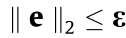 ; the matrix
  is the optimal solution of the coefficient;
  represents all possible solutions; and the definition of norm of
  , where
  is the element of .
The sparsity of the signal is the basic premise in CS theory. Fortunately, most of the vibration signals of civil infrastructure have this characteristic (i.e., the vibration is dominated by a few modes only). Therefore, the vibration data of most structures are usually or almost always sparse in the frequency domain or timefrequency domain. Bao et al. [14] found the sparsity of structural vibration signal and first used the CS for acceleration data acquisition of a bridge SHM system.
Furthermore, the vibration data measured by sensors placed at different locations on a structure have almost the same sparse structure in the frequency domain. Based on the group sparsity of the structural vibration data, a group sparse optimization algorithm based on CS for wireless sensors has been proposed [18]. Supposing that there are  sensors implemented in the structure, the signal matrix
  can be expressed as follows, considering the measurement noise:

where  is the Gaussian noise matrix, is the collected data matrix with
  is a Fourier matrix, and X is a Fourier coefficients matrix. The Fourier coefficients matrix X can then be recovered by solving the following optimization problem:

where  is the zero padding operator and μ is the penalty weight. Once the optimal solution
  has been obtained, the recovered signal matrix can be obtained by the following:

The augmented Lagrange multiplier algorithm is proposed to solve the sparse optimization problem given in Eq. (4) [18]. Fig. 1 shows an example of data-reconstruction results from 10% and 20% measured samples from an actual long-span bridge. Using the reconstructed data, the first two mode shapes can be well identified, as shown in Fig. 2, from the reconstruction signal with 10% samples.
《Fig. 1》
Fig. 1. Data-reconstruction results from (a) 10% and (b) 20% measured samples.
《Fig. 2》

Fig. 2. The first two identified mode shapes from the reconstruction signal with 10% samples.
《3. DL-based anomaly data diagnosis approach》
3. DL-based anomaly data diagnosis approach
Practical experience with a large number of SHM systems has shown that SHM data always contain multiple types of anomalies caused by sensor faults, system malfunctions, and environmental effects. The most common data anomalies in SHM are missing data, minors, outliers, squares, trends, and drifts. These anomalies will seriously shield the real information contained in the data, resulting in a risk of warning misjudgment. Therefore, data preprocessing or data cleaning is important for SHM.
Inspired by actual manual inspection, Bao et al. [50] have proposed a CV- and DL-based anomaly detection method that first visualizes and converts a raw time series into image data, and then trains a deep neural network (DNN) for anomaly classification. The framework of the proposed approach is shown in Fig. 3. This method includes two main steps: ① data conversion by data visualization, in which the time series signals are piecewise represented in the image vector space; and ② DNN training via techniques known as stacked auto encoders and greedy layer-wise training. The trained DNN can then be used to detect potential anomalies in large amounts of SHM data.
《Fig. 3》

Fig. 3. Framework of the proposed data anomaly detection method.
Acceleration data from a long-span cable-stayed bridge was employed to illustrate the performance of the proposed method. Fig. 4 shows the data anomaly distribution identification results over a year. The results in Fig. 4 indicate that the multi-pattern anomalies of the data can be automatically detected with high accuracy, resulting in a global accuracy of 87.0%.
《Fig. 4》

Fig. 4. A comparison between (a) the detection results and (b) the ground truth of the anomaly distribution of acceleration data from a cable-stayed bridge in 2012.
《4. CV-based crack identification algorithm》
4. CV-based crack identification algorithm
CV carries the advantages of less incorporation of expensive professional instruments and sensors, and independence from subjective human experience. By virtue of DL, which automatically trains end-to-end models and generates high-level features of input images, DL-based CV can overcome the limitations of conventional CV, such as the requirement for predesigned filterbased detectors, assumptions about crack geometry, and robustness for complicated real-world images.
Restricted Boltzmann machines (RBMs) and deep convolutional neural networks (CNNs) are two representative DL architectures that have been investigated for image-based crack identification tasks. Xu et al. [51] have established a crack identification framework using RBM for cracks on steel structure surfaces. The proposed RBM model is stacked with an input layer, three hidden layers, and an output layer, as shown in Fig. 5.
《Fig. 5》
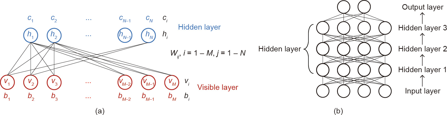
Fig. 5. Schematic of proposed RBM model. (a) RBM with a single visible and hidden layer; (b) stacked RBMs. bi and cj are the offsets and biases associated with the visible vector v and the hidden vector h, respectively, and Wij is the weight related to the unit pair (vi, hj).
RBMs are generative learning modules that can be stacked to form deep networks. An RBM is energy function based and is generally defined as follows:

where x is the input variable of interest, P(x) is the probability distribution with regard to the energy function E(x), and Z is the partition function by traversing all possible inputs. Under some circumstances, the input x can be categorized into the visible and hidden parts (denoted by v and h, respectively). In a Boltzmann machine, the energy function is defined with a second-order polynomial as follows:
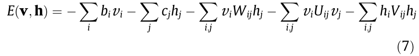
where bi and cj are the offsets and biases associated with the visible vector v and the hidden vector h, respectively, and Wij, Uij, and Vij are the corresponding weights related to the unit pairs (vi, hj), (vi, vj), and (hi, hj). An RBM is defined with its binary units—that is, vi;  . In addition, hj is independent of
  conditional on v and
  is independent of
  conditional on h. Therefore, Uij = 0 and Vij = 0. The energy function of RBM can then be written as follows:

The original images, including complex background information, were taken by a consumer-grade camera (Nikon D7000, resolution: 3264×4928) inside the steel box girder of the bridge. Some of the cracks in the original images are very small, with a width of only a few pixels. Complex disturbance information is also present, such as the edges of steel plates and U-ribs, handwriting by inspectors, electric wires, and corrosion areas. The greyscale 3264× 4928 pixel images were reshaped into an image with the dimensions of 3264×3264 pixels, and then cut into sub-images with the dimensions of 24 ×24 pixels. In total, a complete sub-image set of 240 448 elements was built up. The output label [1 0]T was assigned to crack elements and [0 1]T was assigned to background elements. The input to the deep network was a 576×1 vector reshaped from the corresponding sub-image of 24×24 pixels and normalized by 255 in the grayscale. A contrastive divergence learning algorithm [52] was applied to all the RBM layers in sequence from bottom to top in order to update the weights, biases, and offsets of the stacked network based on the sigmoid function, as follows:
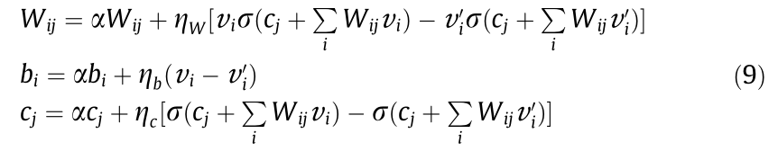
where α and η are the momentum and learning rate hyperparameters. Fig. 6(a) indicates that the reconstruction error ratio decreased to 4.8% after 1000 iterations. Fig. 6(b) shows that the crack elements could generally be differentiated from the disturbance edges, despite the existence of complicated background information.
《Fig. 6》
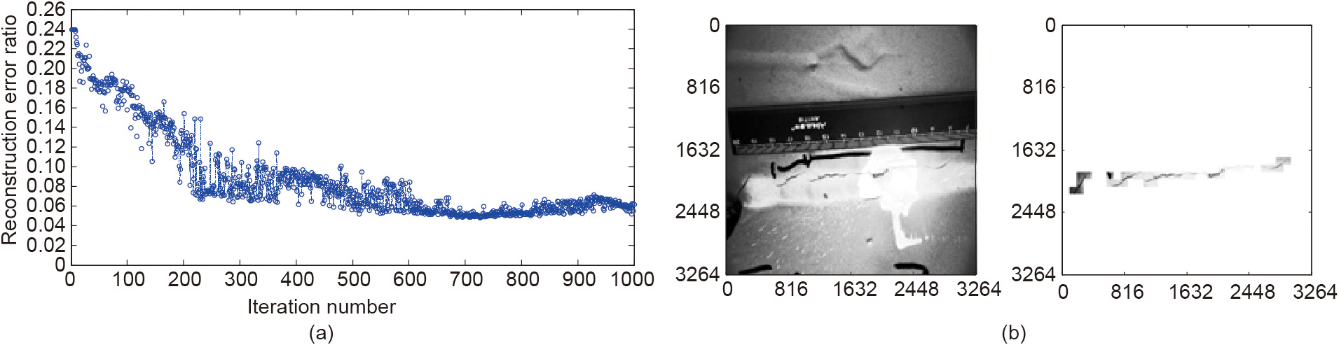
Fig. 6. Results of the training process and crack identification. (a) Reconstruction error ratio; (b) crack identification results.
Inspired by the richer CNN [53], Xu et al. [54] further proposed a modified fusion CNN (FCNN) to handle the multi-level convolutional features for crack identification, as shown in Fig. 7. Unlike the conventional input-hidden-output structure of chain-like CNN, bypass stages are added in FCNN in order to handle the multi-level features. Softmax loss function with a regularization term to penalize large weights was adopted for classification as follows:
《Fig. 7》

Fig. 7. Proposed FCNN architecture and training results. (a) Architecture of the modified FCNN; (b) training and validation recognition errors. Conv: convolution; BN: batch normalization; ReLU: rectified linear unit; MP: max pooling; FC: fully convolution.
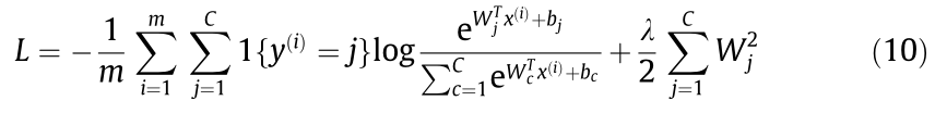
where 1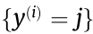 returns 1 if the prediction is correct; otherwise, it returns 0. λ is the weight decay parameter and m represents the mini-batch size. Wj and bj denote the weights and biases in the previous layer, respectively. C represents the total number of categories, and c is the index number ranging from 1 to C;
  represents the ith input of the classification layer;
  and bj represent the weights and biases acting on the ith input ;
  and bc represent the indexes of weights and biases in the internal summation recycle in case of confusion. The recognition error is elementbased and represents the proportion of the predictions missing the ground-truth labels for the input sub-images (i.e., represents whether the prediction of an input element is correct or not). If the predicted label of an input sub-image is different from the ground-truth target label, the number of incorrect predictions is increased by 1 and the recognition error is changed accordingly. Fig. 7(b) shows the training and validation errors during the training process with minimum values of 3.62% and 4.06%, respectively.
Fig. 8 shows the crack identification results of original images taken with different focal distances, in order to validate the performance of the trained network on multiscale images. The figure shows that crack elements are differentiated from the background and from handwriting, even though the latter has crack-like features and acts as a major disturbance for crack identification. The mean value and standard deviation of precision are 88.8% and 6.7%, respectively. The mean value and standard deviation of precision are the statistical results computed over test images under different conditions. The precision is computed in an element-based manner, in terms of whether an input sub-image is correctly categorized as crack, handwriting, or background.
《Fig. 8》

Fig. 8. Identification results of multiscale images. (a) A zoomed-out crack; (b) a zoomed-in crack.
《5. ML-based condition assessment approaches for bridges》
5. ML-based condition assessment approaches for bridges
ML-based condition assessment involves the establishment of a statistical representation of a structure by means of monitored data and assessing whether the condition is normal or not based on changes in the probability density function. For this reason, these methods are also known as pattern-recognition methods.
《5.1. Condition assessment approach for stay cables using ML algorithms》
5.1. Condition assessment approach for stay cables using ML algorithms
Stay cables are crucial members for bridges. However, stay cables suffer from the coupled effects of fatigue and corrosion. Therefore, the condition assessment of stay cables is very important.
The tension force of a stay cable can be monitored by means of a load cell incorporated into the anchorage end of the stay cable. Fig. 9 shows the representative cable tension monitored by load cells in an actual cable-stayed bridge [48].
《Fig. 9》
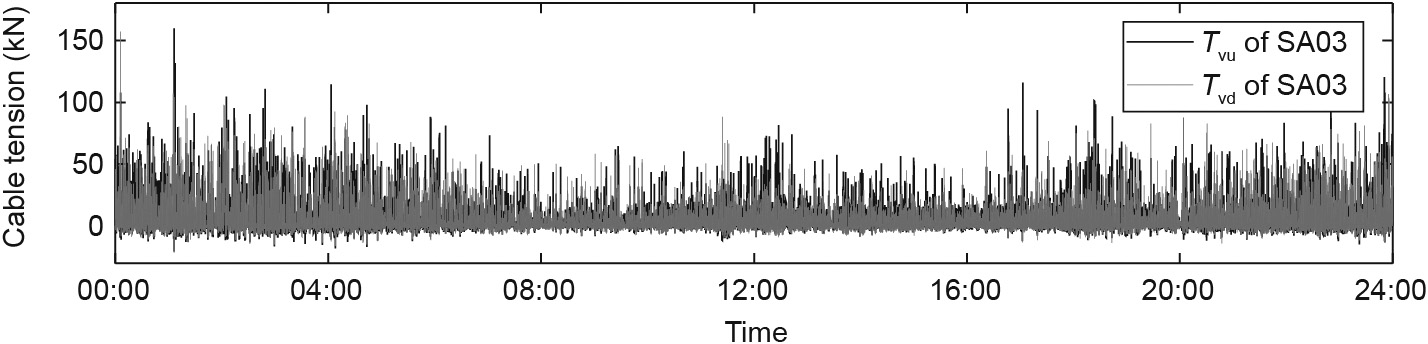
Fig. 9. Monitored tension force of a pair of stay cables. Tvu and Tvd are the vehicle-induced cable tension of the upriver and nearest downriver cables, respectively.
The ratio of the tension force of a pair of stay cables (i.e., the upriver side and downriver side) has been proposed to be as follows [48]:

where  and
and  are the vehicle-induced cable tension of the upriver and nearest downriver cables, respectively;
  denotes the total weight of the loading vehicle, which is assumed to be equivalent to the force loading on the bridge; y is the transverse vehicle position (center of mass); and
  and
and  are the transversal influence lines.
The tension forces of a pair of cables were analyzed using a clustering algorithm [48]; the clustering results are shown in Fig. 10 [48]. It can be seen from Fig. 10 that the ratio of the tension force of the pair of cable is recognizable as six patterns (with different colors denoted).
《Fig. 10》

Fig. 10. Patterns of the tension force of a pair of stay cables. (a) Short cable pair; (b) moderate cable pair.
Further analysis indicates that these patterns are dependent on the transverse locations of vehicles on the bridge only, and are independent of vehicle weight. Once the cables in a cable pair are damaged, the slope (tension ratio) will change. Therefore, the slope of each pattern can be used as an indicator of the condition of the stay cable pair. Cable tension ratio is defined as  . A Gaussian mixture model (GMM) is established, and the parameters of the GMM can be fitted by monitored tension force of a pair of stay cables [48]:

where is the probability density function of the ratio of the tension force of a pair of stay cables m under vehicle n,
  ,
, represents the weight coefficients, and
  .
.
A fitted GMM example is shown in Fig. 11(a), and Fig. 11(b) illustrates the damage detected in an example pair of stay cables [48].
《Fig. 11》

Fig. 11. Condition assessment results for stay cables. (a) Fitted GMM of a short pair of stay cables; (b) contour of a moderate pair of stay cables. PDF: probability density function; CDF: cumulative distribution function; ECDF: empirical cumulative distribution function.
《5.2. Condition assessment approach for a girder using ML algorithms》
5.2. Condition assessment approach for a girder using ML algorithms
The variable of strain links directly to structural safety. However, the welding of a steel girder leaves residual strain and faults in the girder, making it impossible to evaluate the safety of the girder or predict its fatigue life directly using monitored strain. Fortunately, it has been observed that the strain on the top plate of asteel girder has local effects; that is, the amplitude of the strain underneath the wheel of a vehicle on the bridge is very large, and decays sharply with distance. These local effects mean that the strain underneath a wheel is only determined by the wheel load, and is independent from other vehicles on the bridge. The ratio of strains at the same transverse locations, while different sections are independent from the vehicle load, with a time lag (i.e., a vehicle first crosses over one section, and then crosses over another section with a certain time lag). Therefore, the ratio of the strains is related to girder parameters only, and can be used as an indicator of girder condition. The ratio of the strains is defined as follows [49]:
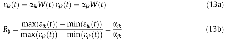
where  and
and  are respectively the strains at the same transverse location (monitored by the kth sensor) of cross-sections i and j when vehicle with the weight of W(t) passing by; and
  and
and  are coefficients that relate to girder parameters only. Thus, the strain ratio
  is only dependent on the structural parameters, can be used as a condition indicator of the girder.
Fig. 12(a) shows the monitored strains at the same transverse locations but at two different sections along a bridge [49]. The similarity of these two strain time histories can be seen. The probability of the ratio of monitored strains at two different sections on the same lane is shown in Figs. 12(b) and (c) [49]. In Fig. 12(b), the parameters of the probability of the ratio of the monitored strain do not change, implying that there is no damage on the girder. In Fig. 12(c), however, the parameters of the probability of the ratio of monitored strain change, indicating the occurrence of damage at these two sections.
《Fig. 12》

Fig. 12. Monitored strain and statistics of the strain ratio. (a) Monitored strain at the same transverse location of two different sections; (b) statistics of the strain ratio without damage; (c) statistics of the strain ratio with fatigue cracking.
《6. Conclusions》
6. Conclusions
This paper provides a brief review of the state of the art of data science and engineering in the field of SHM. Conclusions and future trends are provided below.
A CS-based data-acquisition algorithm is able to randomly sample dynamic signals and reduce the volume of the dynamic signal (e.g., the acceleration, dynamic strain, displacement, etc.) because the dynamic signal in civil structures is sparse in the frequency domain and in the frequency-time domain.
ML, DL, and CV techniques provide efficient algorithms to automatically diagnose anomaly data and perform crack identification and condition assessment using big data from monitoring; they can be extensively applied in SHM.
The concepts of the "automatic AI scientist” and the "automatic AI engineer” are gaining considerable scholarly interest in the field of AI, as they can learn and create theorems, theories, and designs. AI, virtual realization or augmented realization, wearable devices, crowd smart-sensing technology, and their combinations will make it possible to collect more data and information at a low cost, and will lead to novel theories on structural health diagnosis and prognosis by overcoming many challenging issues in traditional damage detection, model updating, safety evaluation, and reliability analysis. These technologies will help us identify a new intrinsic evolution in the long-term performance of full-scale structures in real operational surroundings and under real loads.
《Acknowledgements》
Acknowledgements
This study was financially supported by the National Natural Science Foundation of China (51638007, 51478149, 51678203, and 51678204).
《Compliance with ethics guidelines》
Compliance with ethics guidelines
Yuequan Bao, Zhicheng Chen, Shiyin Wei, Yang Xu, Zhiyi Tang, and Hui Li declare that they have no conflict of interest or financial conflicts to disclose.


 京公网安备 11010502051620号


