

《1. Introduction》
1. Introduction
Modern manufacturing is characterized as high value, low volume, and high customization, and requires zero-defect production management in order to minimize scrap rates and improve product quality and productivity. However, unexpected anomalies (e.g., machining tool breakage, machine spindle failure, or severe tool wear) can cripple the pursuit of the zero-defect target. It is critical to develop effective diagnosis systems to efficiently detect unexpected anomalies during machining processes, and thus permit appropriate adjustments to be made in order to address the anomalies [1,2]. In response to this need, the European Commission has promoted the ‘‘zero-defect manufacturing” concept in manufacturing industries. Accordingly, research projects have been funded in order to identify solutions (e.g., the Intelligent Fault Correction and self-Optimizing Manufacturing systems (IFaCOM) project). From an industrial perspective, some diagnosis systems have been developed and are deployed in factories. A popular strategy in such systems is to identify anomalies by comparing key performance indicators (KPIs) and static thresholds that have been preset by experienced engineers. However, machining processes usually occur under varying working conditions, leading to high dynamics during machining processes. Thus, diagnosis systems that are based on a static threshold setting are unable to address dynamics effectively.
In recent years, smart sensors and cyber–physical systems (CPS) have increasingly been integrated into factories to monitor the dynamic conditions of machining equipment and tooling. As a result, data-driven diagnosis systems have been actively investigated [3–5]. In such systems, intelligent and deep learning algorithms are leveraged in order to mine abnormal patterns from large data streams through time-, frequency-, or time/frequencydomain analysis [6,7]. In order to apply data-driven systems more effectively in industries, it is essential to carry out further research to improve system performance in data processing and analysis.
In this paper, a novel data-driven diagnosis system for computer numerical control (CNC) machining processes is presented. Based on this system, machining processes are continuously monitored to collect data. Analysis is conducted on the monitored data in order to dynamically detect anomalies in the machines and tooling. The innovative characteristics of the system are as follows:
(1) De-noising, normalization, and alignment mechanisms on monitored data have been designed to facilitate anomaly analyses.
(2) A set of features has been defined to represent the most important aspects of the monitored data. Thresholds are used to identify anomalies based on feature comparison. A fruit fly optimization (FFO) algorithm has been applied to optimize the thresholds in order to achieve more accurate diagnosis for dynamic machining processes.
(3) The system has been validated using industrial case studies to prove its effectiveness in practical machining processes.
《2. Literature review》
2. Literature review
In the past, physics- and model-based diagnosis approaches have been the dominant approaches. In recent years, by leveraging the rapid progress that has been made in smart sensors, data analytics, and deep learning technologies, data-driven algorithms have been developed to enhance the effectiveness and performance of diagnosis (e.g., Boltzmann machines, support vector machines (SVMs), convolutional neural networks (CNNs), etc.). Hu et al. [8] developed a method that combined a deep Boltzmann machine algorithm with a multi-grained scanning forest ensemble algorithm to mine faults for industrial equipment. Tian et al. [9] designed a modified SVM to diagnose faults in steel plants; in this method, the data dimension is reduced by a recursive feature elimination (RFE) algorithm in order to speed up computation. Zheng et al. [10] proposed composite multiscale fuzzy entropy (CMFE) and ensemble support vector machines (ESVMs) to extract nonlinear features and classify rolling bearing faults. However, redundant and irrelevant features from data were used, which could reduce the true detection rate significantly and increase the computational time. Wu and Zhao [11] proposed a deep CNN model to detect chemical process faults. However, deep CNN usually requires a high computation time. Madhusudana et al. [12] developed a decision tree technique (J48 algorithm) to detect faulty conditions for face milling tools. In that work, a set of discrete wavelet features were extracted from sound signals by utilizing a discrete wavelet transform (DWT) method. The limit of this research is that the decision tree structure and threshold are difficult to define. Lu et al. [13] proposed a dual reduced kernel extreme learning machine method to diagnose aero-engine faults. Wen et al. [14] proposed a new CNN based on LeNet-5; the proposed CNN was tested for motor bearing, as well as for self-priming centrifugal pump and axial piston hydraulic pump fault detection with an accuracy between 99.481% and 100%. Wen et al. [15] proposed a new deep transfer learning based on a sparse auto-encoder for motor-bearing fault detection with 99.82% accuracy. Wen et al. [16] proposed a new hierarchical convolutional neural network (HCNN), with an accuracy between 96.1% and 99.82%. These works are summarized in Table 1.
《Table 1》
Table 1 Summary of proposed methods.

According to surveys by García et al. [17] and Pan and Yang [18], the following research gaps remain in the further improvement of the efficiency of data-driven algorithms:
(1) It is imperative to design suitable preprocessing technologies for monitored data to ensure the best diagnosis accuracy and efficiency.
(2) Deep learning algorithms usually require a long training time to achieve high accuracy. It is also difficult and costly to acquire sufficient faulty data patterns for algorithm training.
(3) Thresholds to classify different faults are usually preset by experienced engineers. This is not an optimal solution for the increasingly dynamic environments that exist in modern production processes.
《3. System framework》
3. System framework
Power data from the control motors in CNC machines can indicate the working conditions of the machine and tooling [19,20]. Moreover, in comparison with vibration sensors or acoustic sensors [21,22], power sensors are more cost-effective in deployment. Thus, in this system, which is empowered by a wireless sensor network (WSN) mounted onto CNC machines, power data are collected to support anomaly diagnosis of the machine and tooling [5]. The structure of the system is illustrated in Fig. 1. The functions are explained below:
《Fig. 1》
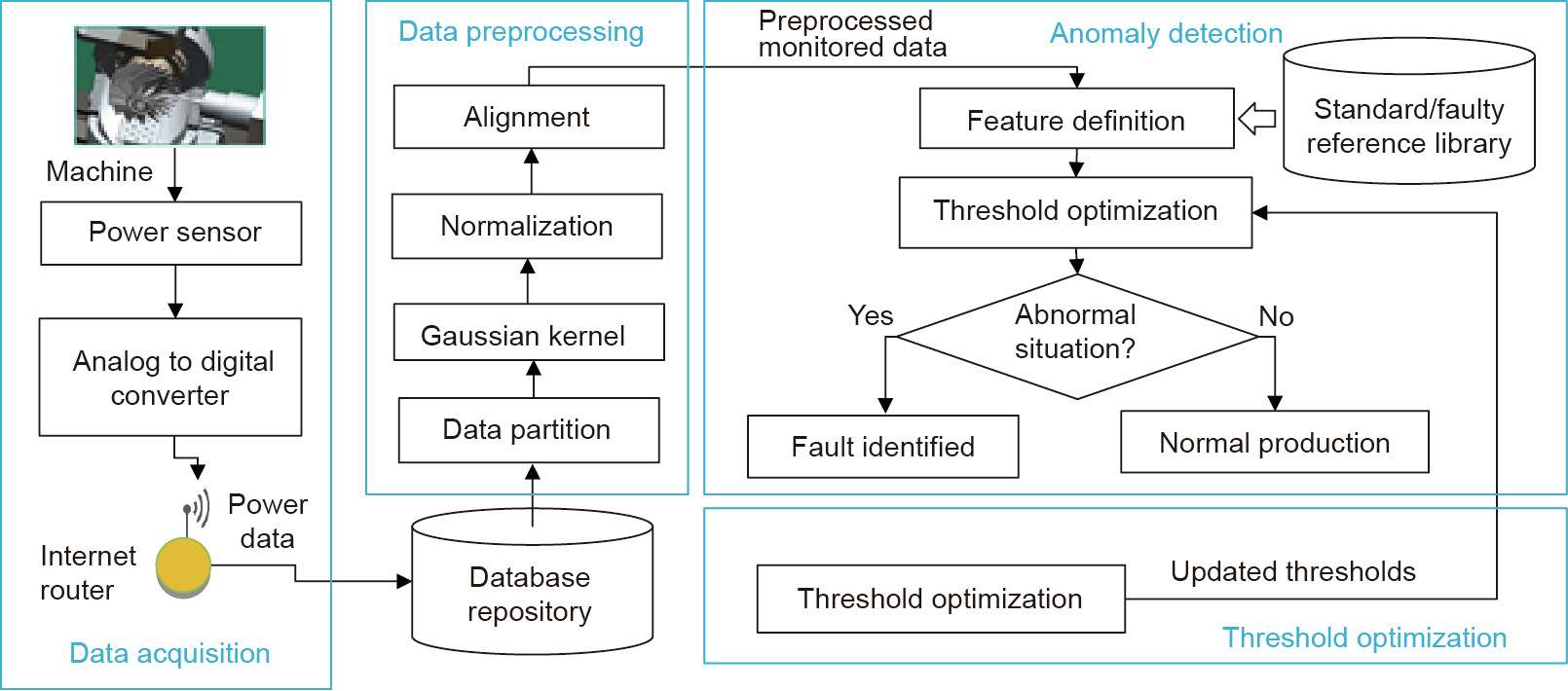
Fig. 1. System framework of CNC machining process.
(1) Data repository: A big data infrastructure has been configured and deployed for collecting, storing, and visualizing realtime monitored data during machining processes [5].
(2) Data preprocessing: Considering the veracity of the monitored data, preprocessing mechanisms have been designed. These mechanisms include: ① Partitioning the data into time-series datasets according to individual machining processes, ② using a Gaussian kernel model [23,24] to de-noise the fluctuated information from the monitored data in order to facilitate further processing, ③ applying normalization to ensure that the scale of the monitored data is suitable for analysis, and ④ performing alignment based on a cross-covariance method [5] to rescale the power data with standard and faculty reference patterns in order to facilitate anomaly identification.
(3) Feature representation and anomaly identification: A set of features has been defined to support anomaly analysis and diagnosis. Thresholds for feature comparisons are used for anomaly identification. The system is open to new anomalies and is dynamically updated during machining processes.
(4) Threshold optimization: An optimization algorithm has been designed to determine optimized thresholds based on historically monitored data.
《4. Preprocessing monitored data》
4. Preprocessing monitored data
《4.1. Partitioning monitored data》
4.1. Partitioning monitored data
Monitored power data acquired during machining processes will be used for diagnosis. Power is calculated based on the following formula:

where  is the ith point of the power data along the time axis
  are the three-phase currents of the power; V is the voltage of the power; and Factor is the quality factor of the power.
It is time-intensive and ineffective to apply analysis on all the power data collected during machining. To facilitate analysis, the monitored data are first partitioned based on machine-specific power levels to represent individual setups of the machining processes. The following steps are then applied on the partitioned monitored data to facilitate analysis further.
《4.2. De-noising and smoothing monitored data》
4.2. De-noising and smoothing monitored data
In general, monitored power data fluctuate as a result of the noises in the signals. In order to extract features effectively, it is essential to de-noise and smooth the monitored data. In this research, a Gaussian kernel-based model is designed for denoising data. The robustness of the Gaussian kernel has been proved by Feng et al. [23] and Rimpault et al. [24]. Here, the monitored data are smoothed by a convolution computation with the Gaussian kernel. The ith point of the de-noised and smoothed power data  is calculated below:

where  represents the total points in
  (the power data);
  stands for the jth point of P along the
  axis (time); and
  is the Gaussian kernel for the jth point with kernel width
An example of the above process is illustrated in Fig. 2.
《Fig. 2》
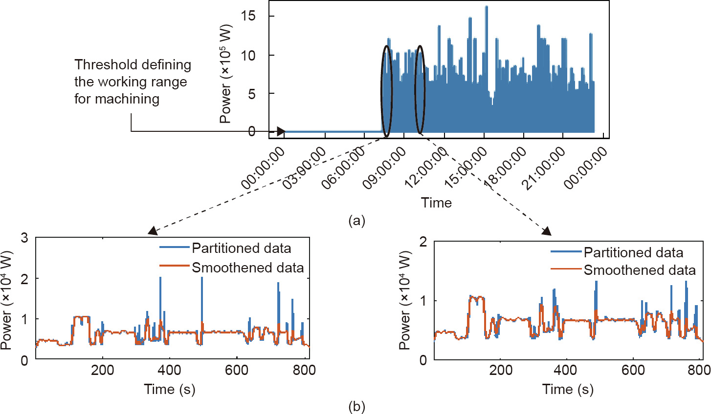
Fig. 2. Example of data partitioning and de-noising of the monitored data. (a) Acquired power data in a single day (31 May 2016); (b) power patterns (in red) for two individual processes after partitioning and de-noising.
《4.3. Normalizing monitored data》
4.3. Normalizing monitored data
Normalization is applied to the monitored data to ensure the proper scale of the data, in order to facilitate feature extraction from the data (e.g., the value of kurtosis, described in Section 5, will be extremely high without the normalization process):

where NP is the normalized power data; is the original power data; and
 is the reference power data of the machine.
《4.4. Aligning monitored data》
4.4. Aligning monitored data
Under practical manufacturing conditions, there may be time delays or deviations in the partitioned monitored data when machining a component, which result in misalignment with a standard reference (i.e., the power pattern when machining the same component under normal working conditions). Cross-covariance between the monitored data and the standard reference (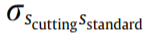 ) is applied to identify the time delay [5].
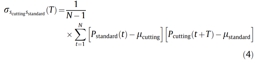
where Pstandard and Pcutting are the standard reference and partitioned monitored data, respectively; μstandard and μcutting are the means of the time-series; N is the smaller number of the two datasets; and t and T are time deviation and standard time, respectively.
The time delay can be calculated by the following formulas:
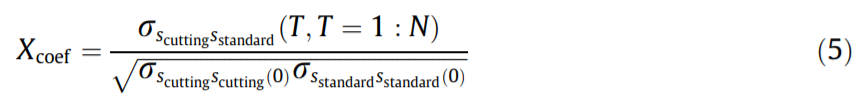
The time difference can be calculated when Xcoef is at its maximum:

Therefore, the aligned monitored data will be:

The same procedure is used to align the monitored data with a faulty reference  (i.e., the power pattern when machining the same component under abnormal conditions) by replacing
  with in the above formulas.
《5. Anomaly-detection process》
5. Anomaly-detection process
During machining processes, Feature is defined to represent the difference between the preprocessed monitored data and the standard reference (i.e., the data pattern of machining the same component under normal working conditions). Standard references are collected during component machining under good working conditions. The diagnosis procedure, which is depicted in Fig. 3, includes the following steps:
《Fig. 3》
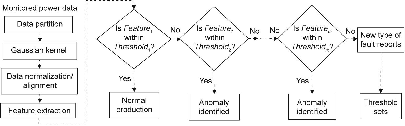
Fig. 3. The anomaly diagnosis process.
(1) Features are represented based on a matrix of the absolute mean, kurtosis, and crest factor. The relevant definitions are provided in Table 2. In Table 2,  is calculated from each piece of preprocessed monitored data and its standard reference.
  are calculated from each piece of preprocessed monitored data and its faulty references (where
  represents an anomaly type).
《Table 2》
Table 2 Definitions of features and thresholds for standard reference, faulty reference, and monitored data [25].

(2) A series of thresholds are defined. Threshold1 is used to determine normal or abnormal conditions by comparing Feature1 and Threshold1. Threshold2–Thresholdm are used to classify the type of anomaly by comparing Feature2–Featurem and Threshold2– Thresholdm, respectively. A new anomaly type will be updated into the database of the system if there is no match of anomalies.
(3) The above thresholds are optimized periodically by an FFO algorithm based on the latest historical data.
In this research, abnormal working conditions are defined based on the following rules [5]:
• Tool wear: Power range shifts vertically significantly, but the power range during the idle stage remains the same.
• Tool breakage: Power increases to a peak value and goes back to the air-cutting power range.
• Spindle failure: Power has a sudden peak and an increased power range during machining and idle stages.
Based on the rules and historical data, three thresholds for the above abnormal conditions can be defined: Threshold2 for judging tool wear, Threshold3 for judging tool breakage, and Threshold4 for judging spindle failure. The process to determine the optimal thresholds is described in the following section.
《6. Threshold optimization》
6. Threshold optimization
As discussed in our previous research [5], the overall detection accuracy can be decided by four factors: True Positive (TP), False Positive (FP), True Negative (TN), and False Negative (FN). TP indicates that an abnormal condition is correctly identified as abnormal; FP indicates that a normal condition is incorrectly identified as abnormal; TN indicates that a normal condition is correctly identified as normal; and FN indicates that an abnormal condition is incorrectly identified as normal. Based on these four factors, Precision, Recall, and F are introduced to evaluate the overall detection accuracy [26]:
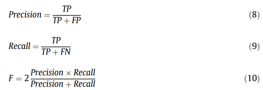
where Precision represents the proportion of correctly identified abnormal conditions against all the identified abnormal conditions; Recall is the proportion of correctly identified abnormal conditions against all the actual abnormal conditions; and F measures the overall accuracy of detection. The higher the F score is (where a good score is close to 1), the better the overall accuracy of detection will be.
TP, FP, TN, and FN are affected by the values of the four thresholds (i.e., Threshold1, Threshold2, Threshold3, Threshold4). Therefore, the value choices of the thresholds affect the F score.
In this research, the thresholds are optimized using an FFO algorithm through historically monitored data rather than by depending on the experience of experts. An FFO is able to avoid local optima, and has better performance than some other mainstream optimization algorithms [27,28]. In this algorithm, swarm centers are initialized to conduct a parallel search (in this research, each center is modeled as a vector of the four thresholds—i.e., Threshold1–Threshold4). Around each swarm center, random solutions called ‘‘fruit flies” are generated. Through smell- and visionbased strategies to calculate fitness and swarm center selection, respectively (details explained in Steps 3 and 4). The computation is iterated toward optimization.
The optimization objective is to identify the most appropriate thresholds that lead to the maximum F score:

The optimization process is described below (improvements to the typical FFO algorithm are provided in Steps 2 and 5):
Step 1. Set the maximum number of iterations Tmax, the population size of the swarm centers v, and the population size of the fruit flies around each swarm center k.
Step 2. Randomly generate fruit flies around each swarm center according to the following formula:

where Vectorcenter and Vectorsub are the vectors of a swam center and of the sub-population of fruit flies around each swarm center, respectively, α is the boundary determining the search distance of the fruit flies around each swarm center, and rand represents a random number.
Step 3. Conduct a smell-based search to calculate the smell concentration (i.e., fitness) for each fruit fly.
Step 4. Conduct a vision-based search to replace the original swarm center with a fruit fly in the sub-population with the best fitness and direct the sub-population to search further.
Step 5. In a typical FFO algorithm, the search distance is always constant, which will make the search difficult to converge when the fruit fly is near to the solution. Therefore, in order to improve the algorithm, the search distance is decreased when the fitness is not improved in five iterations. (This improves the convergence speed, as the swarm can approach the solution in an easier way when the swarm is close to a solution [29].)

where αnew is the decreased search distance when approaching an optimum result.
Step 6. Repeat the steps above until solution convergence or the maximum number of iterations Tmax is reached.
《7. Case studies》
7. Case studies
Sponsored by the EU Smarter and Cloudflow projects, a WSN was developed and deployed on the shop floor of a company in the UK. The company specializes in high-precision machining for automotive, aerospace, and tooling applications. In this case, a five-axis milling machine, MX520, was monitored. For over six months, power data (more than 10 GB) was collected and stored in a local database. A big data infrastructure based on an open source platform, Hadoop, was developed to manage the huge amount of data and to accelerate the data processing.
A part of the production line is illustrated in Fig. 4. Three current sensors (one for each phase) are clamped on the main supply of the CNC machine. The data rate for one sensor is one sample per second; hence, one sample per second is transferred to the Hadoop data server via the Wi-Fi on the shop floor. Power is then calculated based on the three-phase current, the 220 V voltage, and a power factor of 0.82.
《Fig. 4》

Fig. 4. CNC machining processes. (a) Machined part; (b) power measurement; (c) Mazak machine and machining processes.
In this case study, the FFO algorithm was designed to identify the best thresholds leading to the highest F score based on historical data. Table 3 shows the benchmark results for this optimization process. The optimized thresholds are (0.192, 0.032, 0.287) for Threshold1, (0.632, 0.410, 0.652) for Threshold2 as tool wear, (3.698, 75.363, 10.737) for Threshold3 as tool breakage, and (2.412, 1.081, 0.921) for Threshold4 as spindle failure. The FFO algorithm can achieve the optimal result in 23 iterations, and converges the most quickly when compared with other benchmark algorithms. It can achieve an F score of 1, which means that the optimized thresholds can achieve a 100% true detection rate based on the historical data. Some examples of anomaly detection and identification are explained below.
《Table 3》
Table 3 Comparison of optimization algorithms.

GA: genetic algorithms; SA: simulated annealing.
《7.1. Normal production》
7.1. Normal production
Fig. 5 shows an analysis of the monitored data for anomaly detection. The extracted Feature1 is (0.147, 0.004, 0.113), which is smaller than Threshold1 (0.192, 0.032, 0.287) (the definitions of Feature and Threshold are in Table 2). Therefore, it can be classified as normal.
《Fig. 5》
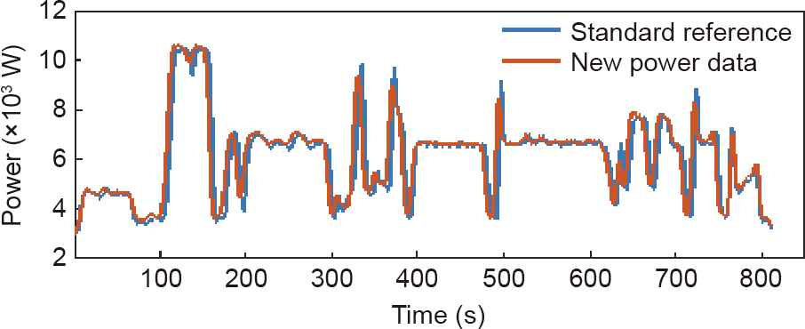
Fig. 5. Monitored data indicating a normal production condition.
《7.2. Anomaly situation: Tool wear》
7.2. Anomaly situation: Tool wear
For the monitored data showed in Fig. 6(a), Feature1 is (0.206, 0.042, 0.295), which is higher than Threshold1 (0.192, 0.032, 0.287). Therefore, the production is classified as a fault. Thus, an anomaly diagnosis is made (Fig. 6(b)). Feature2 is (0.171, 0.058, 0.250), which is smaller than Threshold2 (0.632, 0.410, 0.652). Therefore, the anomaly can be classified as tool wear.
《Fig. 6》
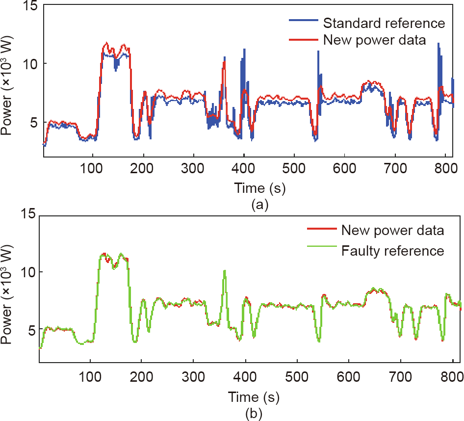
Fig. 6. Tool wear detection. (a) Fault identification; (b) fault classification.
《7.3. Anomaly situation: Tool breakage》
7.3. Anomaly situation: Tool breakage
For the monitored data showed in Fig. 7(a), Feature1 is (0.460, 41.532, 2.303), which is higher than Threshold1 (0.192, 0.032, 0.287). Therefore, the production is a fault. An anomaly diagnosis is made (Fig. 7(b)). Feature3 is (1.039, 61.512, 1.744), which is smaller than Threshold3 (3.698, 75.363, 10.737). Therefore, the anomaly can be classified as tool breakage.
《Fig. 7》
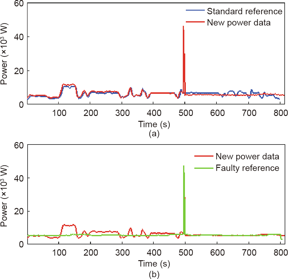
Fig. 7. Broken tool detection. (a) Fault identification; (b) fault classification.
《7.4. New abnormal situation: Long-time air cutting》
7.4. New abnormal situation: Long-time air cutting
Fig. 8 shows an analysis of the monitored data. Feature1 is (0.492, 0.441, 0.379), which is higher than Threshold1 (0.192, 0.032, 0.287). Therefore, the production is a fault. However, there is no faulty reference similar to this data pattern. In this case, therefore, the data was reported to the shop floor engineers. It was found that the machine was accidently left air cutting. The pattern was then saved in order to update the faulty references.
《Fig. 8》
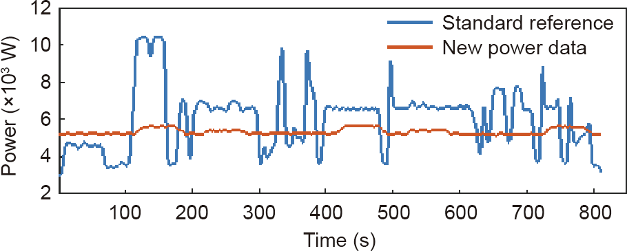
Fig. 8. New abnormal data detection.
《8. Conclusions》
8. Conclusions
In this research, a data-driven anomaly analysis was developed. The system was deployed in a machining company for verification under practical machining conditions. The innovations of this research are as follows:
(1) Preprocessing mechanisms, including de-noising, data normalization, and alignment, were developed to address the veracity issue in monitored data.
(2) An FFO algorithm was designed to identify optimal anomaly thresholds in order to achieve more accurate detection during dynamic machining processes.
Further investigations will be carried out in future to solidify the reliability of the system, including the following: ① A different data sampling rate will be tested to find the best system accuracy and efficiency. Furthermore, different data sources will be considered (e.g., vibration, force data, etc.) by using data fusion to enhance the prediction results. ② We will consider designing effective and efficient deep learning algorithms and computation architectures (e.g., transfer learning algorithms and edge architectures for recurrent neural networks (RNNs) and long short-term memory recurrent neural networks (LSTM RNNs), etc.), to further improve the system performance.
《Acknowledgement》
Acknowledgement
The authors acknowledge the funding from the EU Smarter project (PEOPLE-2013-IAPP-610675).
《Compliance with ethics guidelines》
Compliance with ethics guidelines
Y.C. Liang, S. Wang, W.D. Li, and X. Lu declare that they have no conflict of interest or financial conflicts to disclose.


 京公网安备 11010502051620号


