

《1. Introduction》
1. Introduction
Electron beam selective melting (EBSM) is a typical powder-bed fusion technology that builds parts from discrete powder particles. The geometric freedom enabled by its layer-by-layer building manner [1], its capability for tailoring microstructure [2,3], and its adaptability for certain alloys are among the favorable features of EBSM, in comparison with traditional manufacturing methods. However, this technique also presents a number of challenges. For example, as-built components are subject to void defects, poor surface roughness, and so forth [4,5]. A major cause of these deficiencies is the complicated powder-bed fusion process, which is influenced by multiple processing factors including the beam energy status, scanning strategies, and powder-bed configurations [3,5–7]. In order to investigate the influence of these factors, highresolution numerical models incorporating multi-physics and parameters have been developed, and the single-melt-track formation process has been studied under various conditions [8–10].
The powder-scale mesoscopic simulation model resolves the geometry of discrete particles under multi-physical interactions, utilizing a fine mesh with a size as small as 2 μm and advanced computing algorithms [9–13]. When combined with the powderbed fusion process, fundamental mechanisms such as those of the balling effect and typical surface morphologies can be revealed [9–11]. Furthermore, in situ observations of the powder-bed fusion process with a high-speed camera and high-energy X-rays have been incorporated in order to validate the mesoscopic models [14–16], and the deposited melt tracks from experiments have been compared with simulation results and show an overall agreement [9,13,17].
When applying the mesoscopic simulation approach to investigate the melt track deposition process, various morphologies of the deposited melt tracks can be generated under different processing conditions. In general, these morphologies can be categorized using visual classification into, for example, continuous lines, semicircle droplets, and separated agglomerations, based on the explicit geometrical characteristics of the simulation results [13]. However, qualitative classification cannot depict the variety of melt tracks precisely, or establish a numerical relationship between the process parameters and the melt track morphologies. Thus, there is a need for an informative characterization method for melt tracks that can reflect most geometric features and distinguish the marginal difference under similar processing parameters. A simple and effective idea is to transfer visual-based classification into quantified geometric indexes of melt tracks.
This paper first proposes strategies for defining and extracting the characteristic geometrical values of simulated melt track morphologies. Major descriptive indexes for the melt track geometric dimensions are obtained and correlated with specific surface morphologies. Furthermore, the relationship between the processing parameters and the extracted geometric data is investigated. The effects of different parameters and potential defects, as indicated by extracted melt track data, are addressed. Finally, a simulation-driven optimization framework is proposed that utilizes the tools of mesoscopic simulation, data extraction, and machine learning; this framework can assist in exploring the processing window in an intelligent way.
《2. Method and setting》
2. Method and setting
《2.1. Mesoscopic simulation》
2.1. Mesoscopic simulation
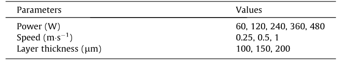
Mesoscopic modeling of EBSM has been developed in our previous work [9,18]. The full energy equations of a powder bed under electron beam (EB) irradiation have been solved, with the resolution of discrete particle geometries, and key physical phenomena such as surface tension and recoil pressure have been included. Details of the numerical implementation of the multi-physical mesoscopic simulation can be found in the related literature; this paper focuses on the quantification of geometric data from the simulation results. Single-track deposition processes under various processing conditions are simulated. The investigated processing parameters, which include energy power (P), scan speed (v), and layer thickness, are listed in Table 1. There are five different values of energy power, three different values of scan speed, and three different values of layer thickness, making a total of 45 processing conditions.
《Table 1》
Table 1 Different sets of power, speed, and layer thickness.
Ti–6Al–4V powder particles in the range of 40–100 μm are generated on a substrate using the discrete element method (Fig. 1(a)), and the initial temperature of the powder bed is set at 900 K, considering the preheating effect. The simulation domain is 3000 μm × 800 μm × 600 μm and is meshed with a uniform 8 lm grid, which can efficiently reduce the computing cost without a substantial loss of accuracy. The material properties of Ti–6Al–4V are given in Ref. [9].
《Fig. 1》

Fig. 1. (a) Initial setup; (b) simulation results of the powder-bed melting process.
《2.2. Identifying the melt track》
2.2. Identifying the melt track
After the single-track mesoscopic simulation is completed, the powder-bed morphology with a solidified melt track is obtained, as shown in Fig. 1(b). When employing the volume of fluid (VOF) method to calculate the free boundary flow of the melting pool, the variable volume fraction F is introduced to represent the interface between the fluid (F = 1) and the void (F = 0), as shown in Fig. 2(a) [19]. Therefore, by detecting the F values in each cell and its neighboring cells, the geometric boundary of the powder bed—that is, the surface morphology—can be captured. In the current model, the simulation domain is discretized into  grid cells (Fig. 2(b)), corresponding to a three-dimensional (3D)
 matrix. By constructing the isosurface of the F matrix, the deposited powder-bed surface morphology can be obtained, as illustrated in Fig. 1(b).
《Fig. 2》

Fig. 2. (a) F representation of the free boundary dimensional F matrix; (b) 3D F matrix of the simulation domain.
In order to better understand the melt track characteristics, we will modify the F value to only show the deposited melt track instead of the whole powder bed. To extract the melt track, the unmelted parts/cells are excluded by setting their F value at 0. Whether or not a cell is melted depends on the temperature history: If the temperature value never exceeds the melting point, then a factor of 0 is assigned to the cell, while melted parts are assigned a factor of 1. The final 3D F matrix value is obtained by multiplying the F matrix and the factor in each cell. In this way, the isosurface of the melt track is constructed, as shown in Fig. 3(b).
《Fig. 3》

Fig. 3. Extracting a melt track from the powder bed. (a) The powder bed after melting; (b) the extracted melt track.
《2.3. Defining geometric quantities》
2.3. Defining geometric quantities
Based on the extracted melt track in Fig. 3, geometric dimensions such as width and height can be measured. As mentioned above, the matrix of F indicates the distribution of materials in each cell. Therefore, the width or height of the melt track is measured by counting the number of cells with non-zero F values. To be specific, the matrix is first projected into horizontal and vertical planes, which correspond to the  and
and  -shaped matrices. Next, by connecting the outmost non-zero cells, the geometric boundary can be constructed, as shown in Fig. 4. The width of the melt track is defined as the sum of the distances from the left
 and right
  boundary to the beam center (Fig. 4(a)). The height of the melt track is defined as the distance between the upper boundary and the top surface of the substrate. The depth of the melt track is defined as the distance between the lower boundary and the top surface of the substrate (Fig. 4(b)). These geometric values are measured cell by cell along the melt track length, and are stored in arrays that can be manipulated to reflect the fluctuation of these geometric quantities.
《Fig. 4》
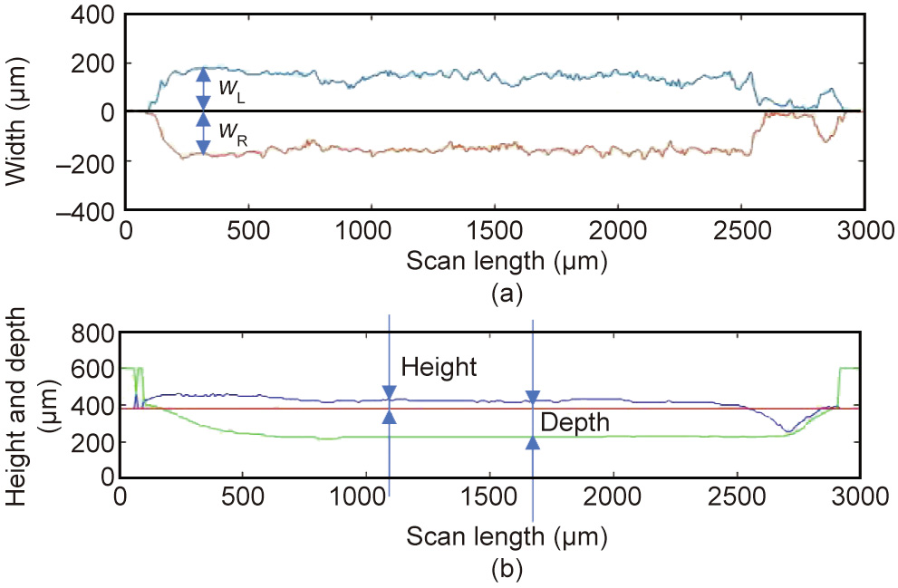
Fig. 4. Definition of the melt track’s geometric profiles.
《3. Results and discussion》
3. Results and discussion
《3.1. Geometric description and quantification》
3.1. Geometric description and quantification
To validate the effectiveness of the previously introduced approach for quantifying the geometric features of melt tracks, three representative melt track morphologies—a narrow line, a bold line, and a wavy line—are selected from the simulation conditions in Table 1. The powder beds of these three types of melt track after simulation are shown in Fig. 5. The extracted melt tracks and the measured width distributions are shown in Figs. 6 and 7, respectively.
《Fig. 5》

Fig. 5. Finished powder beds for different processing conditions: (a) P = 60 W, v =1m·s-1 ; (b) P = 240 W, v = 0.5 m·s-1 ; (c) P = 480 W, v =1m·s-1 .
《Fig. 6》

Fig. 6. Extracted melt tracks for different processing conditions: (a) P = 60 W, v =1m·s-1 ; (b) P = 240 W, v = 0.5 m·s-1 ; (c) P = 480 W, v =1m·s-1 .
《Fig. 7》
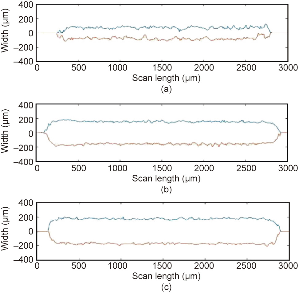
Fig. 7. Widths of melt tracks for different processing conditions: (a) P = 60 W, v =1m·s-1 ; (b) P = 240 W, v = 0.5 m·s-1 ; (c) P = 480 W, v =1m·s-1 .
Comparing the finished powder beds in Fig. 5 with the extracted melt tracks in Fig. 6 and the measured widths in Fig. 7 results in an overall agreement, except for the case of the wavy melt track in Fig. 5(c). The melt track in Fig. 5(c) has a necking morphology that is not reflected in Fig. 7(c). In this case, the method for measuring the melt track width is not reliable for representing the actual morphology. To explain this effect, a cutting plane vertical to the melt track length is employed to illustrate the shape of the melt track in the width direction, as shown in Fig. 8. The yellow part indicates the melt track shape.
As stated above, the width defined as  in Fig. 8 corresponds to the outmost boundary in the horizontal direction. This definition overestimates the melt track width, as few materials are deposited near both ends above the substrate top surface (the horizontal line in Fig. 8). A more reasonable strategy is to take the width of the materials above the top surface of the substrate (
 in Fig. 8) as the effective width. The modified width distribution is shown in Fig. 9, and generally matches the morphology in Fig. 5(c).
《Fig. 8》
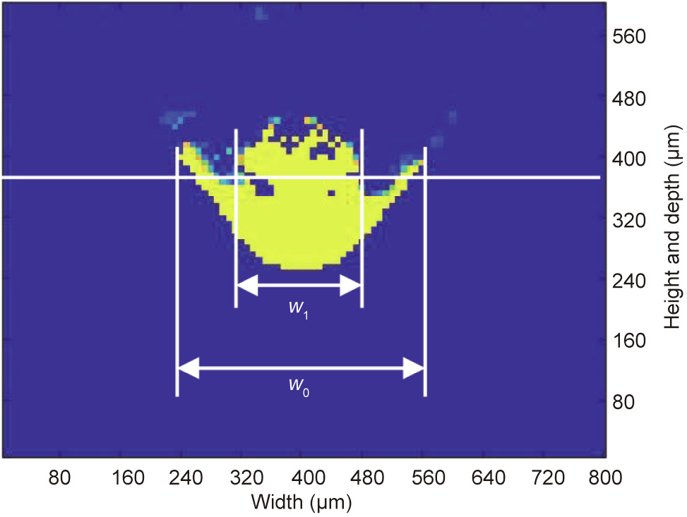
Fig. 8. Melt track shape vertical to the scan direction.
《Fig. 9》
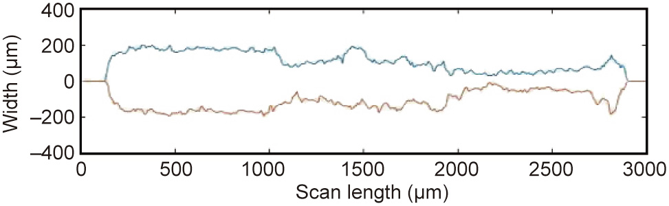
Fig. 9. Updated melt track width using the definition of .
The extracted melt track profiles make it possible to quantitatively describe the geometric features through statistical analysis of the measured dimensional values, as indicated in Table 2. The variables  in Table 2 stand for width, height, and depth of the melt track, respectively, as defined in Fig. 4; the abbreviations ave and std refer to the average and standard deviation values, which indicate the geometric size and fluctuation levels. The standard deviation values of the depth for the three processing conditions are small and are therefore omitted. In order to exclude the effects of discontinuities at the start and finish of a melt track, only the central part (1000–2000 μm) is measured.
《Table 2 》
Table 2 Geometric quantities for different processing conditions (unit: μm).

As expected, the values in the seven columns in Table 2 are in accordance with the surface morphologies shown in Fig. 5, which can be regarded as indicators of the deposition quality. For example, the negative value of the melt track depth d for the condition of P = 60 W, v =1m·s-1 indicates the occurrence of a lack of fusion, which also comes with a narrow width, as depicted in Fig. 5(a); in addition, the large value of std w or std h for the condition of P = 480 W, v =1m·s-1 indicates the occurrence of flow instability, which is depicted as the necking morphology in Fig. 5(c). This agreement proves the effectiveness of the defined qualification approach, and paves the way for subsequent data-based analysis and optimization.
《3.2. Experimental verification》
3.2. Experimental verification
The experimental verification work is carried out on a self-developed EBSM machine from QBEAM (QuickBeam Tech. Co., Ltd., China). Single-track depositions are performed with the parameters listed in Table 1. The powder particles used are Ti–6Al–4V in the range of 40–100 μm, and the powder layer thickness is 75 μm. Instead of depositing single tracks as the first layer on the substrate, a rectangular box is first built until the layer thickness converges to a steady value. Two typical deposited melt track morphologies, along with the corresponding simulation results, are shown in Fig. 10.
《Fig. 10》

Fig. 10. Melt track morphologies for the parameters of P = 480 W, v =1m·s-1 (top) and P = 240 W, v = 0.25 m·s-1 (bottom) from (a) experimental and (b) simulation results.
The experiment results show general agreement with the simulation results. With a large power and scan speed (P = 480 W, v =1m·s-1 ), the melt track width becomes fluctuant and necking is observed, caused by fluid instability; in comparison, with a medium power and speed (P = 240 W, v = 0.25 m·s-1 ), a straight and bold melt track is formed. Considering that there are uncertain factors such as the powder stacking condition, beam power size and shape, powder-bed temperature, and so forth, which differ in the experimental and simulation settings, the results from the mesoscopic modeling can be regarded as reliable in reflecting complex melt track morphologies under different processing conditions.
《3.3. Data analysis》
3.3. Data analysis
The dependency of melt track morphologies on the processing parameters has been a key issue for the quality control of EBSM. Now, based on the extracted geometric data of melt tracks, it is possible to determine these relationships quantitatively. Three major parameters—namely, the energy power, scanning speed, and layer thickness, as shown in Table 1—are investigated. Four of the seven descriptive indexes from Table 2—namely, ave w, ave h, std w, and std h—are extracted for different parameter values, as illustrated in Fig. 11.
《Fig. 11》

Fig. 11. Melt track size for different scan speeds and powers. Average value of (a–c) melt track width and (d–f) melt track height, and standard deviation value of (g–i) melt track width and (j–l) melt track height for layer thickness of (a, d, g, j) 100 μm, (b, e, h, k) 150 lm, and (c, f, i, l) 200 μm.
Fig. 11 shows 12 individual plots, including four rows of plots corresponding to the ave w, ave h, std w, and std h values of the melt tracks, and three lines of plots corresponding to the layer thicknesses of 100, 150, and 200 lm, respectively. In each plot, the x-axis is labeled as different power values, and three different colors represent the different speed values. For ease of comparison, the y-axis range is kept the same for different layer thicknesses. Some data points—such as the parameter set of P = 480 W, v = 0.25 m·s-1 —are not plotted in the figure because they are regarded as ‘‘overmelt,” as the energy input is so high that the calculated melt pool depth exceeds the geometry boundary (3000 μm × 800 μm × 600 μm). For this condition, the measured depth is incorrect and is therefore excluded. Also, some data points—such as P = 360 W, v = 0.25 m·s-1 in Fig. 11(g)—are invisible due to the std w value exceeding the y-axis range.
The grey part in each plot is set to distinguish data points with acceptable width and height values. The basic principle for judging the melt track quality is that the ave w and ave h values are as large as possible while the std w and std h values are as small as possible, as these conditions can enhance the overlapping and reduce the fluctuation of melt tracks. Therefore, for some points outside the region—such as points P1 in Fig. 11(a) and P2 in Fig. 11(l)—the melt track quality and processing parameters can be regarded as unsuitable. In this way, the extracted melt track quantities guide the selection of suitable processing parameters.
When looking further at the distributions of the data points, it can be observed that an increase in layer thickness shifts the processing parameter window toward a larger energy input, as more points stay in the right side of the grey region (Fig. 11). This trend can be simply explained by the fact that a larger layer thickness indicates more powder, and thus requires more energy to melt. The energy density represented by the ratio of power to speed, P/v, affects the melt track geometry by either changing the power or scanning speed: Considering the different color lines/speeds in Figs. 11(a–f), when the scanning speed increases, the melt track width decreases and the height increases; considering the same color line for different powers, when the energy power increases, the melt track width and height first increase and then decrease for a smaller layer thickness. It can be found that the melt track geometries are not simply affected by the energy densities, but are more affected by specific parameters.
The formation of melt tracks is directed by melting pool dynamics. Normally, a high energy density results in a large melting pool size and hence a large width or height. However, there are some conditions under which this relationship does not apply. For a small layer thickness, increasing the power (i.e. increasing the energy density) over a certain value will reduce the width, as indicated by Fig. 11(a). The underlying mechanism for the width decrease under high energy levels can be attributed to the effects of fluid flow and evaporation, as illustrated in Fig. 12. Normally, the melting pool under the EB is drilled and later refilled by the backwards flow, as shown in Figs. 12(a–c). However, when the energy density is extremely large, the evaporation and recoil pressure cause a greater penetration depth, which cannot be fully compensated later before the boundary of the melt track solidifies. Under these conditions, the width value measured will have decreased, as shown in Figs. 12(d–f).
《Fig. 12》

Fig. 12. Melt track width decrease at high energy levels. (a–c) Evolution of a normal melt track width; (d–f) evolution of a reduced melt track width.
In addition to the melt pool dynamics, the layer thickness evidently influences the melt track geometry. Fig. 13 illustrates the melt track contour for different powers with a layer thickness of 100 and 200 μm, respectively. It can be observed that for a larger layer thickness, the melt track height does not increase; instead, it decreases slightly with increased input power, which is revealed as the tendency in Fig. 11(f). This tendency occurs because at a greater layer thickness, a lower input power does not sufficiently melt the powder close to the substrate; therefore, the solidified melt track is deposited above this unmelted powder. However, as the input power increases, the powder near the substrate fully melts, resulting in enhanced layer shrinkage and a smaller height. For a small layer thickness, the input power is sufficient, and no unmelted powder is left below the melt track. When the input power value increases, more materials melt and the curvature of the top surface of the melt track is enlarged, which leads to a larger melt track height (Fig. 13(c)). However, with a high input power, the melt track decreases, as indicated by Fig. 12(f).
《Fig. 13》

Fig. 13. Melt track geometry for different layer thicknesses and powers. (a–c) Melt track geometry for a power of 120, 240, and 360 W, respectively, and a layer thickness of 100 μm; (d–f) melt track geometry for a power of 120, 240, and 360 W, respectively, and a layer thickness of 200 μm. Black line: the boundary of the melt pool.
Thus far, the influences of the energy density and layer thickness—which correspond to the amount of heat and materials—on the melt track morphology have been illustrated. However, the scan speed, as related to the heat conduction and dissipation time, is another significant factor that remains to be investigated. In order to illustrate the effects of the scan speed upon constant energy density, the data in Fig. 11 are re-arranged with scan speed as variable and energy density kept constant, and replotted in Fig. 14 . The contents are similar in comparison with Fig. 11, except that different color lines represent different energy densities. It can be observed that for the same color line—that is, the same energy density—almost every plot shows a positive relationship between the speed and the geometric variables. This trend can be comprehended from three aspects: ① For the standard deviation value of the width or height, a higher speed is likely to result in flow instability which eventually develops into fluctuant melt track morphologies. ② At a constant energy density, a higher speed indicates greater power. Although the interaction time is reduced, the beam can still melt the powder bed instantly within this short period. Considering the Gaussian distribution of beam power, a large power value results in a larger zone above the energy threshold that can melt the powder bed, as indicated in Fig. 15. ③ Even when the energy density remains the same, when the scan speed decreases, the deposited energy is more likely to dissipate to the substrate or the as-built layers, resulting in lower efficiency in melting the powder and, therefore, a smaller melt track size.
《Fig. 14》

Fig. 14. Melt track size for different scan speeds and energy densities. Average value of (a–c) melt track width and (d–f) melt track height, and standard deviation value of (g–i) melt track width and (j–l) melt track height for layer thickness of (a, d, g, j) 100 μm, (b, e, h, k) 150 lm, and (c, f, i, l) 200 μm.
《Fig. 15》

Fig. 15. Illustration of increased melt track width with increased energy power.
Finally, a brief data sensitivity analysis of the relationship between three of the above-mentioned parameters and the melt track geometrical dimensions is conducted to assess the significance of each parameter. The one-factor-at-a-time (OFAT) method [20,21] is used, and the sensitivity value (S) is obtained by calculating the ratio between the relative change of the melt track dimension and the relative change of the processing parameter corresponding to two neighboring sample points, as indicated in the following equation:
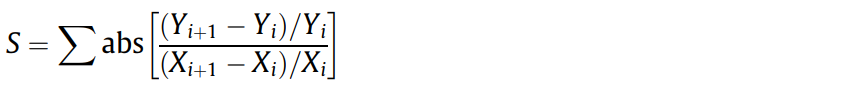
where abs represents calculating the absolute value of the expression in the bracket, Y represents the melt track geometry, X represents the processing parameter, and i is the sample point number.Three parameters are investigated—namely, power, speed, and layer thickness—and three individual values for each are included (although the energy powers of 60 and 480 W are neglected), resulting in a total of 27 sample points. The results are listed in Table 3.
《Table 3》
Table 3 Data sensitivity between the processing parameters and melt track geometry.
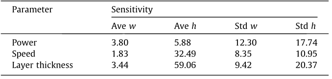
As a very preliminary exploration of the sensitivity level for different parameters with a limited number of sample points, it is inferred that energy power is the most dominant factor in determining the melt track width, and that layer thickness is the most dominant factor in determining the melt track height. The impact of scan speed is less important. Considering the contribution in the expression of energy density, P/v, the energy power P as the numerator is linear to the energy density, while the scan speed v as the denominator is inversely proportional to the energy density, which is less sensitive for a larger scan speed. The melt track height, as analyzed before, is governed by several mechanisms such as coalescence and shrinkage. The significance of the energy power and scan speed rank differently for ave h and std h, which remains to be understood further.
《3.4. Simulation-driven optimization framework》
3.4. Simulation-driven optimization framework
Thus far, we have combined the mesoscopic simulation model with the data quantification method and applied them to research the effects of power, speed, and layer thickness on melt track morphology. With a high-fidelity simulation model and representative indexes of the extracted melt track geometry, the quality of the melt track can be assessed in an efficient way. Based on this foundation, a simulation-driven optimization framework is proposed. A schematic is shown in Fig. 16. Since most of the simulation and data-processing work can be executed under predefined settings, it is feasible to set batches of sample simulations and generate a massive database under different processing conditions. Machine learning or data mining techniques can be utilized to reveal the relationships between processing inputs (power, speed, etc.) and outputs (melt track width, height, etc.) once these data are prepared. With the obtained relationships, various processing conditions can be predicted prior to simulations or experiments, and an optimized processing parameter window can be built, which can save a great deal of time and work. Furthermore, after establishing comprehensive knowledge of the relationships between the processing inputs and outputs for a single-track case, this method can be introduced to instruct real conditions involving interactions between multiple tracks and multiple layers, which are more closely related to the generation of processing defects.
The idea depicted in Fig. 16 is at an early stage but shows a great deal of potential, as it replaces massive trial-and-error experiments with automatic explorations using computers. However, some issues still remain to be figured out, including: ① the accuracy and credibility of the current simulation model, which still lacks detailed experimental validation; ② the standardization of the melt track geometrical information, such as the definition and measurement of geometric features; and ③ the massive computing cost, which is a great challenge thus far, and restricts engineering applications. In the near future, the work depicted in this paper will be extended to cover more simulation samples under different processing conditions, enrich the database for the framework, and show more practical values.
《Fig. 16》
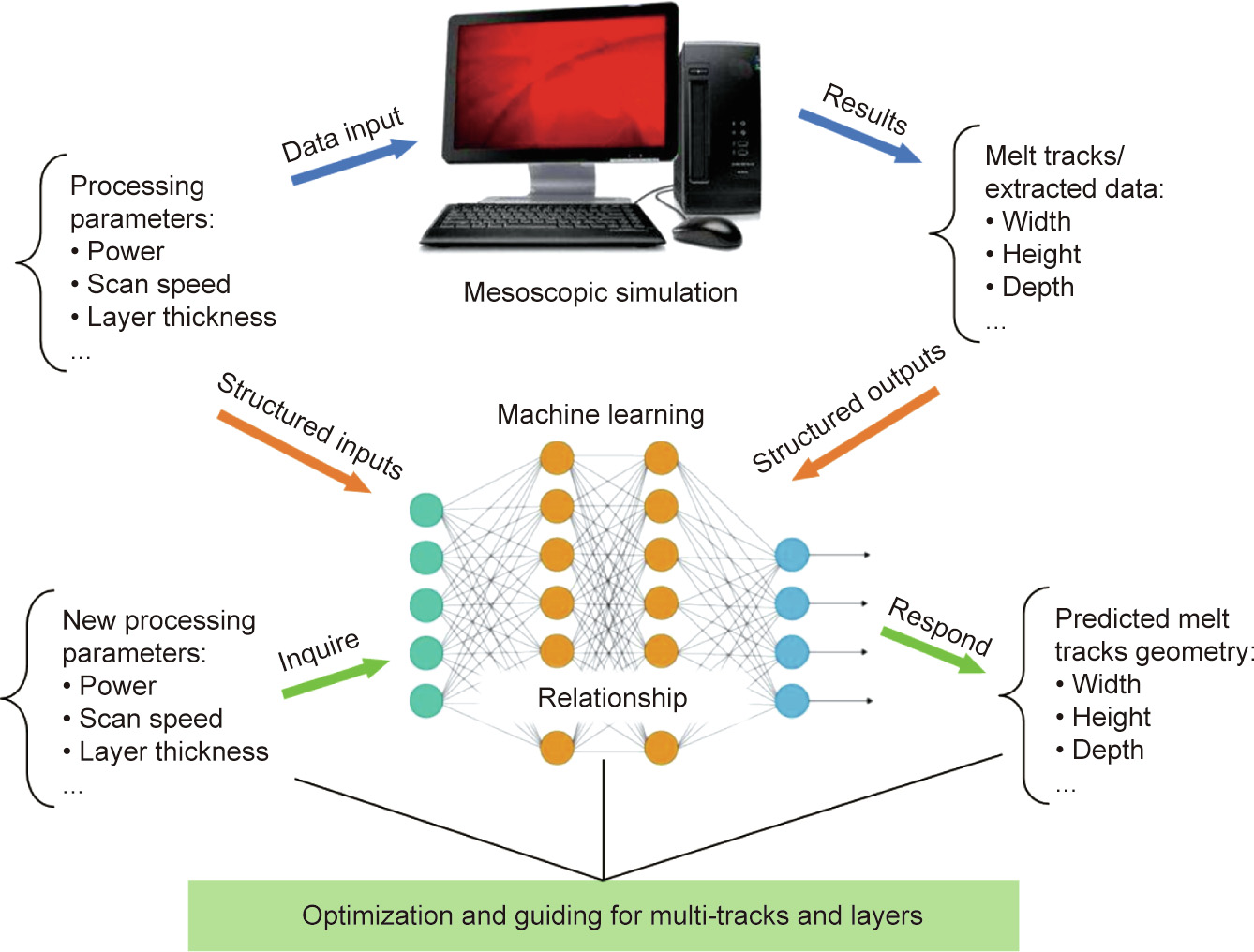
Fig. 16. Roadmap of the simulation-driven optimization framework.
《4. Conclusion》
4. Conclusion
This paper develops a numerical approach to simulate and assess the EBSM process. Together, the mesoscopic model and the results quantification method can reflect the deposited melt track morphology under different processing conditions. Using the numerical approach, the effects of energy power, scanning speed, and layer thickness on the melt track geometries are investigated. The results of this research suggest a simulation-driven optimization framework that is capable of exploring suitable processing windows via computing.
《Acknowledgements》
Acknowledgements
Ya Qian and Feng Lin acknowledge financial support by the National Key R&D Program of China (2017YFB1103303) and the Suzhou–Tsinghua Special Innovation Leading Action (2016SZ0216). Wentao Yan would like to thank the Singapore Ministry of Education Academic Research Fund Tier 1 for its support.
《Compliance with ethics guidelines》
Compliance with ethics guidelines
Ya Qian, Wentao Yan, and Feng Lin declare that they have no conflict of interest or financial conflicts to disclose.


 京公网安备 11010502051620号


