
《1. Introduction》
1. Introduction
In recent years we have witnessed a rapid surge of interest in novel person-based sensing devices, for example, for wellbeing, sports, safety, childcare, healthcare, and bio-surveillance [1]. In parallel, an additional aspect increasingly moving into the forefront is the mobile environmental monitoring by individual-worn sensors combined with a smartphone [2]. Intelligent sensors (called smart sensors) accomplish the acquisition of an electric signal from a physical property as well as the processing (and storage or communication) of measured signals, an amenity that makes them excellent personal exposure recorders. The wearable environmental sensors approach pools the recordings of environmental data (air quality, temperature, humidity, radiation, noise, etc.) together with recordings of human activity spaces [3]. The latter represent the urban areas within which people move during the course of their daily activities and that can be tracked by Global Positioning System (GPS)-devices [4].
The role of personal exposure in the etiology of environmental (and often chronic) health problems was emphasized by the exposome concept [5] that attributes high importance to an individual’s exposure compared to their genetic make-up. Epidemiological studies of environmental health effects often work with data aggregated at regional levels. Statistical associations are studied between disease prevalence or incidence in certain districts and data of environmental parameters gathered at fixed monitoring stations that are ‘‘representative’’ for each of these districts (often based on administrative boundaries). However, recordings from a sparse station network do not adequately represent the range of exposure experienced by different individuals, especially in diverse indoor and outdoor urban environments [6].
Moreover, while results from such studies are valid for the given scheme of districts, they change for another arrangement of districts which is known as the modifiable areal unit problem (MAUP) [7,8]. Therefore, more advanced approaches focus directly on individuals and work with buffers around the individuals’ residences. Applying ecological regressions, these studies analyze the associations between the individuals’ health status and the percentages of traffic, green area, industrial area and so on in their buffer as surrogate measures for exposure [9]. Evidently, the real personal exposure of each individual is only indirectly measured with this approach and exposure misclassification occurs that can weaken the statistical significance of the results [10,11].
As a remedy, individual-worn sensors can record environmental parameters directly at a person’s location; some authors call it anthropocentric opportunistic sensing [12]. The small size of modern sensors, their smart functionality, and affordable costs make them perfect tools to register exposure data in vivo. Our commentary aims to guide the choice of appropriate sensors, to improve the understanding of obtained results, and to highlight the principal needs of constructive elements of wearable environmental sensors (Fig. 1). In particular, we outline standards for application procedures of these sensors. Such standard operating procedures (SOPs) depend on the intended purpose of the study and the research question. The illustration through examples and challenges is an attempt to initiate more interdisciplinary discussions related to constructive elements and diverse use of sensors and wearables in environmental monitoring, public health, and personal exposure assessments.
《Fig. 1》
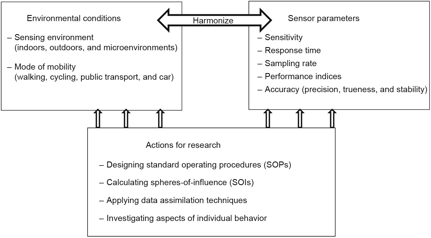
Fig. 1. Short facts of environmental sensing by individuals.
《2. Utility of person-worn environmental sensors》
2. Utility of person-worn environmental sensors
Personal exposure is multifactorial, involving, for example, air temperature, air humidity, radiation, air pollutants (gases, particulate matter), and noise. This definition aims to encompass all exogenous exposure factors contributing to the human exposome.
As the health outcome or discomfort associated with an exposure depends on the vulnerability and the behavior of an individual, additional person-specific variables have to be considered. They comprise fixed values (e.g., age, sex, and pre-existing health conditions) as well as time-dependent values (e.g., movement behavior recorded by GPS and breath rate that is related to physical activity recorded by accelerometers [13]). Smartphonebased sensing methods have become a valuable way to simultaneously collect many of these variables [14,15].
Individual-based environmental measurements are useful for two very different purposes. First, they continuously collect complete exposure data for an individual. This approach results in metrics for cumulative exposure, location and activity-specific exposure increments, frequency distributions of exposure increments [16], mobility habits, and behavior. It can facilitate behavioral changes and adaptation for a sensor wearing individual and being informed about its current exposure status. At the very least this can help to promote individuals’ environmental health literacy [17]. For example, cyclists can adjust their travel behavior according to information assigned to their geo-position [18,19]. Second, individuals can act as urban explorers and, by means of their portable sensors, can capture the variability of atmospheric parameters [20]. Combining such crowdsourced measurements from numerous people, or with model simulations, data for all locations/times in the city are estimated within a participatory citizen science approach [21,22]. Plotting the spatiotemporal data along the trajectory of each person (according to the concept of time-geography [23]) can improve the understanding of disease prevalence, etiology, transmission, and treatment [24]; and also help to support sustainable urban planning.
《3. Concepts of personal exposure measurements》
3. Concepts of personal exposure measurements
Environmental exposure relevant to a person’s health has to be locally monitored constantly for the individual. The results of such continuous monitoring suggest different levels (and combinations) of exposure depending on the individual’s immediate surroundings [25]. Due to this concept, the exposure associated with the daily agenda of a person is a sequence of pollution patterns, each characterizing a specific microenvironment. For example, black carbon exposure was found to be significantly elevated in diesel vehicles, in the subway, or rooms with environmental tobacco smoke [26].
This microenvironment concept facilitates an approximate exposure estimation based on an individual’s time–activity profile and characteristic pollution levels of the involved microenvironments [25]. Typical microenvironments are homes, schools, and vehicles for transit/commuting [27]. Exposure to outdoor pollutants occurs not only outdoors, but also indoors in naturally ventilated homes [28]. While, in the past, the microenvironment was categorized according to activity logs (diaries) or geographic proximity [29], and the utilization of GPS and accelerometers allows for automated human activity recognition [3,30].
A weakness of this microenvironment concept is that indoor air pollution varies considerably between different apartments and only very general information is available for selected typical set tings. Further, outdoors and especially in urban neighborhoods, the pollution can vary considerably due to many potential sources (e.g., industry and traffic) and rapidly changing dispersion conditions in street canyons. For example, studying the PM2.5 (particulate matter with an aerodynamic diameter no greater than 2.5 μm) exposure of schoolchildren, Rabinovitch et al. [31] observed relatively high correlations between the mean concentrations in the microenvironments of home, transit, and school. This raises the question of variability between and within microenvironments. Only very few individual exposure records show clear differences between microenvironments. Much more pronounced are concentration peaks that occur independently of the microenvironment. The authors identify these peaks (exposure events) as an exposure metric that is associated with health effects.
Another concept of personal exposure is linked with the urban structure. Here the basic assumption is that land use is a proxy for climatic, air quality, and noise conditions. Land use regressions (LURs) are used for modeling [32]. The assumption is valid under weak wind conditions (autochthone weather) and also (but weaker) as an average over long periods (in the sense of long-term climate). Mobile personal measurements can provide valuable data for LUR models in high spatial resolution complementing stationary monitoring if appropriate cross-validating schemes are applied to estimate the predictive model performance [33].
《4. Sampling points and sampling rate》
4. Sampling points and sampling rate
Conventionally, the (urban) atmosphere is monitored by a network of meteorological and air quality stations that are placed at fixed locations with the aim of gathering representative data. For an appropriate selection of these locations, guidelines have been developed [34]. However, the urban environment is strongly inhomogeneous and influenced by numerous different processes and the selection of these representative sites is a challenge. One important aspect for the site-selection is the rationale of monitoring: Does it aim to collect climatological data or is it intended to provide data in support of particular needs, such as the prevention of health problems? This determines whether the immediate vicinity (e.g., a street canyon), the neighborhood, or the entire city is the scale of observation.
To specify the optimum number and disposition of climatologic monitoring sites in an urban area, information about meteorological scenarios representative of the considered region is usually combined with spatial simulations of pollutant concentration patterns or even composite air quality indices [35]. The sum of all these air quality patterns weighted by the probabilities of their occurrence results in the figure-of-merit (FOM). Its maxima help to identify and rank the most desirable monitoring locations. The lowest number of optimal locations are characterized by non-overlapping spheres-of-influence (SOIs), determined by a cut-off value in the spatial autocorrelation between the pollution level at this site and the neighboring monitoring sites [36,37].
While semi-variances assess the spatial autocorrelation structure of the entire pollution field (and can be useful for the spatial interpolation of pollution data [38]), the SOI concept is based on the calculation of correlograms that are specific for each location. The correlogram cut-off distance (usually after a correlation decay by 1/e (≈ 36.8%) indicates the size of the region for which the recordings are representative. We suggest the transfer of this concept to mobile measurements and to use it for the sampling rate specification. If the SOIs of a sequence sampled during a walk overlap (see example in Fig. 2), the sampled values are correlated because the sampling points are too close together. That means larger time periods between the individual samples can be selected; in other words, sampling rate, which is the number of samples per hour, can be reduced.
《Fig. 2》
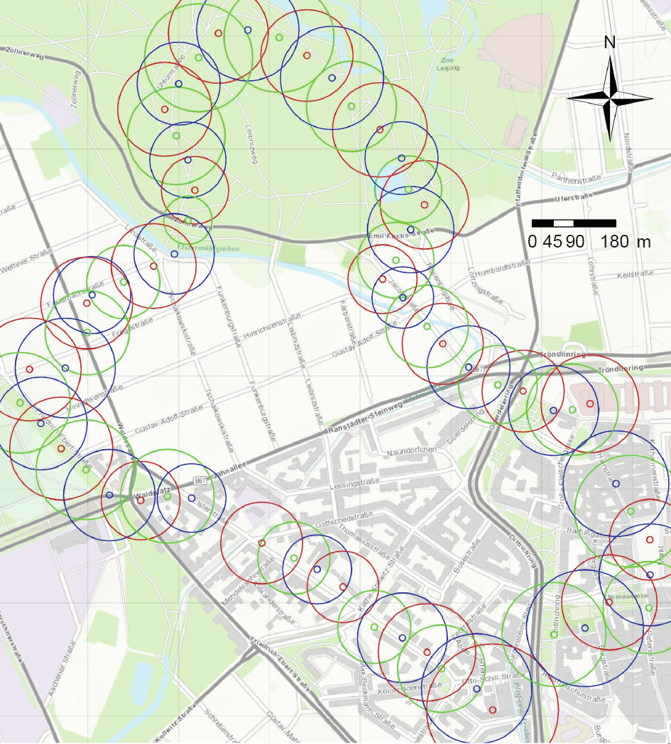
Fig. 2. Spheres-of-influence (SOIs) calculated from mobile temperature recordings sampled with a ventilated (55 m·s-1 flow rate) and sun-protected sensor (data logger testostor 171 with humidity/temperature probe 0572 6172, Germany; accuracy: ±0.2 K,  ≈ 12 s ( is the time constant characterizing the duration a sensor will need to respond to a step-input)) 1.5 m above ground during a walk made 22:50–00:00 UTC on Tuesday, 18 July 2017, in Leipzig, Germany. The dots mark the sampling sites (coordinates registered by a GPS (Garmin GPSMap 60CSx, USA), which are separated by a time-step of 1 min. The circles around the dots mark the SOI-distance at which the correlation of temperature in the center with the remaining data decays by 1/e (≈ 36.8%) (exponential function fitted to the correlogram; negative correlations removed). The sampling rate was 5 s, so that for each sampling site 12 recordings (comprising 1 min) were included into the correlation calculation. The daily temperature profile was estimated using a lowpass filter (6 h cut-off period) and then eliminated from the recordings. To improve readability, successive circles were plotted in colors red, blue, and green. The urban structure is visible in the background (coordinate system World Geodetic System 1984 (WGS84), Universal Transverse Mercator (UTM) zone 32).
《5. Accuracy of sensors—A matter of performance》
5. Accuracy of sensors—A matter of performance
An important issue of miniature sensors is their accuracy. While equipment for condition monitoring (e.g., temperature/humidity control in factories or pollutant monitoring in mines) aims at the detection of extreme values, a sensor that gathers personal environmental burdens has to register very low concentrations with high accuracy [39], which involves ① high precision (small random fluctuations and good repeatability), ② trueness (no bias from the true value), and ③ stability (no long-term drift). Trueness can be achieved by regular calibrations, but precision and stability are immanent to the measurement technique. For that reason, not every technique is suitable for application in wearable environmental sensors.
Regular calibration of the sensors according to the manufacturer guidelines is a must. The field measurement performance can be evaluated by comparison with a standard high-end instrument [40]. A set of indices is available for the assessment of the sensors’ precision: index of agreement [41,42], Pearson’s correlation coefficient, root mean squared error, mean bias error, mean absolute error, and coefficient of variation. When multiple factors are simultaneously sampled, a similar accuracy of all sensors is desirable. This will guarantee that each factor measurement has the same reliability at a sampling point. In practice, the sensor accuracy can be assessed from a comparison with a precision instrument by means of Bland–Altman and Taylor plots [40].
《6. Time constant of a sensor》
6. Time constant of a sensor
Another important parameter is the time constant , characterizing the duration a sensor will need to respond to a step-input (more precisely, 1 – 1/e (≈ 63.2%) of the step-value). Considering that the sensor might be carried during a walk with a speed of approximately 5 km·h-1 (≈ 1.4 m·s-1 ) and the environmental conditions markedly vary within a range of 14 m, an adequate sampling rate needs to be 10 s. The sensor has to be compatible with this sampling rate and the time constant has to be ≥ 10 s (unfortunately, many of the new smart sensors have ≤ 1 min). The time constant essentially depends on whether or not the sampling is active (that means sensor ventilation by a micro-fan using a standardized flow rate is applied). In contrast, passive sampling is generally not adequate in the context of mobile measurements as to the large time-constant (inertia effect). An example comparing active and passive temperature measurements (Fig. 3) demonstrates that considerable mismeasurement can result from an inappropriate combination of sampling rate and time constant.
《Fig. 3》
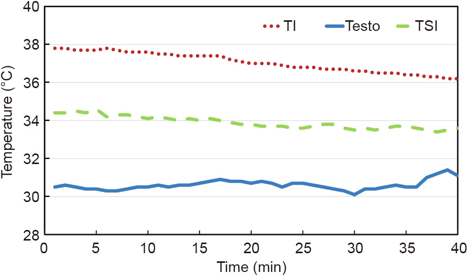
Fig. 3. Contemporaneous recordings of different temperature sensors and sampling modes (outdoor temperatures gathered at time steps of 1 min): Testo Sensor (data logger testostor 171 with humidity/temperature probe 0572 6172, Germany; accuracy: ±0.2 K, ≈ 12 s) active sampling with sun protection and ventilation; TSI Q-Trak 7565 sensor (USA; accuracy: ±0.6 K, ≈ 30 s) handheld with natural ventilation and no sun protection; Texas Instruments (TI) SensorTag CC2650STK (USA; accuracy: ±0.2 K, ≈ 300 s) without any sun protection and ventilation.
Undoubtedly, in a specific application of a wearable sensor, the sampling rate needs to be adapted to the existing spatial variability of the environmental parameter (see the SOI concept above), the speed of the mobile measurements, and the sensor’s time constant. Possibilities to tune the sampling rate may be limited—not every sensor is useful to every design for personal environmental monitoring.
《7. Implementation of personal monitoring》
7. Implementation of personal monitoring
The arguments above suggest that the implementation of mobile measurements depends on their purpose and the prevalent environmental conditions. The variability of the environmental parameters can be assessed by point measurements, geostatistical techniques (e.g., semi-variogram analyses), and micrometeorological modeling. For the measurement task at hand, it will be very helpful to develop an SOP, which is state-of-the-art with pharmaceutical and industrial processes.
Such an SOP for mobile measurements involves a detailed description of the measurement procedure, including the purpose of the study, materials and devices, details of the sensors (including functionality, energy supply, calibration, accuracy, and time constants), details on the implementation of mobile measurements (flow diagram), a protocol for the mobile measurement campaign (including start date and time, location, preparations required for the measurements, sampling rates, carriers (e.g., pedestrians, bikers, and cars)), average movement speed, sampling period, method of synchronization between all sensors and GPS, potential sources of errors, data storage details, and data analysis approaches. Such working instructions are useful for researchers that test different sensors and novel devices or explore the environmental conditions near urban hot spots. They are vital for high-quality population studies when laypeople carry wearable sensors during everyday life and record their burden for health studies. Templates, as well as planning tools, are available for support [43].
A manual acquisition of all the collected data would be tedious and therefore the data stream has to be integrated and rapidly processed within a data acquisition system linking sensors, smartphones, and a database [44]. An important task of this data processing is the synchronization of all measurements that is usually based on a timestamp [45]. Future developments toward an Internet of Things (IoT, as a global data infrastructure [46]) can bring data management to perfection and simultaneously increases data accuracy and coverage [47]. For example, shortdistance communication techniques like iBeacon↑ (↑ http://www.ibeacon.com/.)can improve the registration of positions in an indoor environment and contribute to a comprehensive assessment of indoor and outdoor environmental burdens.
《8. Upvaluation of sensor records》
8. Upvaluation of sensor records
All data recorded by wearables are subject to considerable noise [48]. Small scale turbulence near the person, nuisance of recordings due to impacts (e.g., heat, acoustic noise, and trace gases) caused by the moving individual, and other perturbations will generate outliers as well as bias in the measured data. The quality of the recorded data can be enhanced when an urban region is ‘‘explored’’ by numerous individuals. During their movement, the data collected at nearby points in time and space can be averaged for random noise reduction. A systematic technique that interpolates many such measurements is the so-called data assimilation, which combines measurements with micro-meteorological simulations. This approach is similar to the procedure that is operationally applied to meteorological and climatological measurements on a global scale.
Because measurements always have uncertainty, the data assimilation procedure needs to take this into account for the calculation of the combined data and their uncertainty. As an adequate solution for this task, we suggest the Bayesian spatiotemporal epistemic knowledge synthesis [49]. This approach can combine micro-meteorological simulations (of air pollutants, temperature, etc.) with multiple person-carried measurements resulting in highly resolved data of environmental parameters and their confidence intervals.
Another perspective of wearable sensors is the association of recordings with the perceptions of the carrier. A novel technique registering a person’s apperceptions during their daily life are walking interviews [50]. Being in a certain urban setting, people are more easily able to reflect their own experiences and this mirrors the measured environmental conditions. This technique is derived from ethnographic studies and can bridge between measured exposure data, an individual’s behavior, and their health status. In combination with wearable sensors, the walking interviews can uncover daily habits and the social context as determinants of personal exposure and contributors to the etiology of chronic diseases. Smartphone sensing methods are a feasible way to integrate active user feedback (e.g., exposure perception) on the move [45].
《9. Conclusions》
9. Conclusions
Novel sensor and information technology developments can contribute considerably to the provision of human exposome data [51] and foster the transition from population-based to individualbased epidemiological studies [52]. While some environmental parameters are reflected by human perceptions (such as the thermal comfort and noise), others are basically imperceptible (such as particulate matter and NOx concentrations). As a corrective, multifactorial exposure measurement can immediately inform a person about prevalent health risks [53]. This is especially important for epidemics of non-communicable (e.g., asthma and diabetes) as well as communicable (e.g., tuberculosis and coronavirus disease 2019 (COVID-19)) diseases, that are influenced by people’s everyday lifestyle and surrounding environments. Further, wearables can help overcome the microenvironment and land-use concepts that are not individual-based. However, the application of wearable sensors demands specifications for sampling rate, accuracy, and numerous other conditions, ideally in the frame of an SOP (Fig. 1). To avoid spurious and biased recordings, the sensors themselves must actively sample (i.e., ventilated by a micro-fan) and be protected against the impact of nuisance parameters. Combining individual-based records with environmental modeling as well as novel techniques surveying ‘‘on the move” are promising challenges for future research activities.
《Acknowledgements》
Acknowledgements
The work was partially supported by the German Research Foundation (Deutsche Forschungsgemeinschaft, DFG) under Schwerpunktprogramm (SPP) 1894 ‘‘Volunteered Geographic Information: Interpretation, Visualization and Social Computing”, project ‘‘ExpoAware—Environmental volunteered geographic information for personal exposure awareness and healthy mobility behavior” (SCHL 521/8-1). The authors acknowledge the help of Niels Wollschläger with the calculation of SOIs (Fig. 2).


 京公网安备 11010502051620号


