《1. Introduction》

1. Introduction

Process monitoring is necessary and meaningful for industrial systems, and attracts a considerable amount of attention from both industry and academia [1–4]. In general, process-monitoring methods are divided into three categories: the model-based approach, the knowledge-based approach, and the data-driven approach [5–8]. The model-based approach uses a mathematical representation of the system and thus incorporates a physical understanding of the system into the monitoring scheme. The knowledge-based approach uses graphical models such as PetriNets, multi-signal flow graphs, and Bayesian networks (BNs) for system monitoring and troubleshooting. This approach is especially well-suited for the prognosis of coupled systems [9]. The data-driven approach for monitoring does not require reaction mechanisms or first-principles knowledge of the process. In recent years, by leveraging the rapid progress that has been made in smart sensors, data analytics, and deep learning technologies, the data-driven approach has been developed to enhance the effectiveness and performance of diagnoses [10]; advances in this area include Boltzmann machines, support vector machines (SVMs), convolutional neural networks (CNNs), and more [11–13]. Recently, data-driven methods have become the mainstream of complex industrial process monitoring.

However, most data-driven methods currently assume that the historical training data and the online monitoring data follow the same distribution [14–16]. In fact, the collected data from real industrial processes are always affected by many factors, such as the changeable operating environment, variations in raw materials, and production indexes [17]. These factors often lead to problems such as model mismatching when the model that was learned based on training data is applied to actual online monitoring. Such problems make it difficult to achieve accurate process monitoring. In order to resolve the problem of historical training data and online testing data following different distributions, pioneering works have been proposed. Hou et al. [18] proposed an incremental principal component analysis (PCA) online model for timevarying process monitoring. In this model, when a new sample is obtained, the PCA model is updated by the original PCA model and the new sample, the squared prediction error (SPE), and the T2 limits are updated as well. Jiang et al. [19] proposed a multimodel discriminant partial least-squares (DPLS) method based on the current data and historical data to diagnose the data. Zhang et al. [20] established a deep belief network (DBN), which had a strong generalization ability, to monitor welding status online. In order to adapt to the addition of new data samples, Zeng et al. [21] proposed an incremental local preservation projection (LPP) algorithm, which is updated by using the Laplacian matrix and the projection value of the original sample. However, these algorithms cannot cope with the large difference between two domains that occurs when, for example, the monitored industrial process is located in a completely different operating environment. Ge and Song [22] proposed the online batch independent component analysis–principal component analysis (ICA–PCA) method, in which new data is monitored using a fitted ICA–PCA model selected from the model storeroom. However, this method requires the construction of multiple models, and unbalances in data will reduce the monitoring performance.

Dictionary learning usually involves learning an over-complete dictionary; then, the raw data can be reconstructed by a dictionary and a sparse matrix. Real raw data usually possess the characteristic of structural redundancy. Through dictionary learning, the raw data are mapped to a lower dimensional space, which removes the structural redundancy of the raw data while simultaneously retaining the most concise information. Peng et al. [23] proposed a method that worked out a mapping dictionary through LPP in order to retain the geometric structure of the raw data. Chen et al. [24] proposed a method that utilized dictionary regularization to create a dictionary that learned from a small amount of target domain data; this dictionary was similar to a dictionary that learned from the source domain data. Zhang et al. [25] proposed a method in which a common dictionary, a source domain dictionary, and a target domain dictionary were learned in order to realize crossdomain classification. In the method proposed by Jie et al. [26], several subspace dictionaries between the source domain dictionary and target domain dictionary were learned. Long et al. [27] proposed a transfer sparse code (TSC) that introduced graph regularization and reduced the distribution distance in order to realize knowledge transfer. These dictionary learning methods have made great achievements in signal reconstruction, signal noise reduction, image recognition, image correction, and other aspects, which have attracted a great deal of attention in both academia and industry. Moreover, recent studies have shown that dictionary learning has an extraordinary advantage in process monitoring. Huang et al. [28] proposed a kernel dictionary learning method to achieve nonlinear process monitoring and a distributed dictionary learning method to achieve high-dimensional process monitoring.

Although the abovementioned methods exhibit superior process-monitoring performance in industrial systems, they do not take the distribution divergence of historical data and online monitoring data into account. Transfer learning, which is a general framework for knowledge transfer in different domains, has been extensively investigated in recent years, especially in the communities of artificial intelligence, image recognition, and computer vision. Inspired by the powerful representation ability of dictionary learning and the cross-domain knowledge-transfer ability of transfer learning, a robust transfer dictionary learning (RTDL) method is herein proposed to deal with the problem of the distribution divergence of realistic industrial process monitoring. The proposed method is a synergy of representative learning and domain adaptive transfer learning. To summarize, historical training data and online testing data are separately treated as the source domain and target domain in the transfer learning problem. For an industrial system, although the system always operates in different operating environments, which inevitably results in different data distribution, the underlying internal information, such as the mechanism, is often the same or similar. In other words, the high-dimensional observation data of an industrial system often have invariant subspaces in different domains. Therefore, it is feasible to map the source domain and the target domain to a common subspace, in which the distribution difference between the source domain and the target domain is eliminated. After that, process monitoring is carried out in the learned subspace. For practical use, a discriminative dictionary learning method is proposed to extract features from multimodal industrial data. Next, maximum mean discrepancy (MMD) regularization [29] is proposed as a nonparametric distance metric to express the distribution distance, which reduces the distribution divergence between the source domain data and the target domain data. In addition, in order to reduce the distance of the interior mode data, linear discriminant analysis (LDA) regularization is introduced. Accordingly, the proposed method can learn a robust common dictionary even if the source domain and target domain are seriously affected by a different operating environment; thus, this method can effectively improve the performance of process monitoring and mode classification.

The main contributions of this paper are summarized as follows. First, an RTDL method is proposed to reduce the negative effect of an industrial system’s changeable operating environment. By reducing the inter-domain differences, the proposed model can reduce the performance degradation of process monitoring and mode classification caused by a changeable operating environment. Second, detailed optimization steps about the constrained nondifferentiable dictionary learning problem are given, which can efficiently solve the RTDL problem. Third, the proposed method is verified by extensive experiments, including a numerical experiment and real industrial experiments. The results demonstrate that the proposed method can outperform some state-of-the-art methods in accuracy; thus, this method is suitable for the task of process monitoring industrial systems.

The rest of this paper is organized as follows. Section 2 briefly introduces domain adaptive transfer learning, dictionary learning, and the motivation for this paper. In Section 3, the RTDL model is proposed and its effective optimization steps are given. In Section 4, extensive experiments including a numerical simulation, the continuous stirred tank heater (CSTH) benchmark case, and a wind turbine system case are conducted to verify the effectiveness of the proposed RTDL method. Finally, Section 5 provides a conclusion and summary remarks.

《2. Preliminaries》

2. Preliminaries

《2.1. Domain adaptive transfer》

2.1. Domain adaptive transfer

Suppose that there are a source domain with a large amount of data,   (where n s is the number of source domain data ), and a target domain with a small amount of data,   (where n_t is the number of target domain data ). Here, the source domain and target domain are related but not the same. Taking a wind turbine system as an example, set the process data of the wind turbine system in winter as the source domain and set the process data in summer as the target domain. These two domains are related, since the data of each domain are collected from the same wind turbine system under the same mechanism. However, due to the external operating environments being different, the observation data from the two seasons often have different distributions. Mathematically, the input feature space of the domains is the same, but the marginal distribution and conditional distribution of the domains are different; namely,  , and  , where P_s and P_t represent the probability distribution of source domain and target domain, respectively; represents data space; x represents the data sample; and y represents the label of the data x.

In order to achieve process monitoring in the target domain, it is necessary to eliminate the distribution divergence between the source domain and the target domain—namely, the conditional distribution difference and the marginal distribution difference. When the distribution divergence of the source domain and the target domain is eliminated, the source domain data can show the same process information as the target domain data, so the method can take advantage of abundant source domain data to aid the training model, and thus achieve a positive knowledge transfer effect.

《2.2. Dictionary learning》

2.2. Dictionary learning

The philosophy of dictionary learning is to minimize data reconstruction errors by learning a dictionary composed of a series of atoms and a sparse matrix. Let 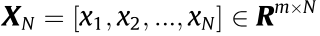 be the set of raw samples, where x_N represents the Nth sample with a dimension of m, m is the number of data dimensions, R is the vector space, and N represents the amount of data.  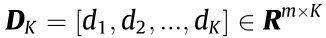is a dictionary composed of K atoms, where d_K is the Kth atom and K is the number of atoms.  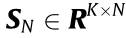stands for the sparse matrix. The problem of dictionary The problem of dictionary learning can be expressed as follows:

where α ( α > 0) is a parameter to control the sparsity of S_N ,  represents the F norm of the matrix and  represents the L₀ norm of the matrix S_N .

《2.3. Motivation》

2.3. Motivation

As mentioned earlier, although an industrial system may operate under different operating environments (e.g., due to external interference such as different locations, time, weather, and manual operation), which inevitably results in a divergence in the data distribution, the underlying internal mechanisms are often the same or similar to each other. That is, the high-dimensional observation data of an industrial system under different domains often have invariant subspaces. Therefore, it is necessary to extract the invariant knowledge or subspace in order to eliminate the extrinsic interference and thereby further enhance the performance of industrial process monitoring.

In order to show the effect of the transferable feature between the source domain data and target domain data vividly, Fig. 1 shows a scatter diagram of data that are influenced only by different environmental factors that cause different distributions. The marginal distribution and conditional distribution of the source domain and target domain are obviously different. The traditional data-driven method has two common strategies: As shown in Fig. 1(a), the first strategy is to ignore the source domain data and only use the target domain data as the input data, so as to meet the assumption that the distribution of the training data is the same as the distribution of the testing data. However, because there is very little training data in the target domain, the final model is prone to overfitting. As shown in Fig. 1(b), the second strategy is to ignore the different characteristics of the source domain and the target domain. This strategy uses a large amount of historical data and a small amount of new data directly to conduct the model training task; thus, the final model confuses inter-domain difference information with abnormal information. Moreover, it is easy for the model to be dominated by the source domain, which has a large amount of samples. In contrast, Fig. 1(c) shows the RTDL model proposed in this paper. This method attempts to find a mapping relationship function . Through this mapping relationship, the raw data are mapped into a subspace. In this subspace, the marginal distribution and conditional distribution of the source domain are the same as those of the target domain; that is,   and   (where   is the mapping with respect to x). We believe that if can overcome the interference of the extrinsic environment and only keep the most concise internal mechanism information, it can transfer knowledge from the source domain to the target domain. That is, by incorporating MMD and LDA-like regularizations into the dictionary learning objective function, the proposed method can take advantage of the abundant source domain data to aid the training model and achieve the transfer effect, in order to improve industrial process monitoring.

《Fig. 1》

Fig. 1. This figure depicts a situation with a large amount of source domain data and a small amount of target domain data. (a) Traditional strategy 1 ignores the source domain and only utilizes the target domain data for model training. (b) Traditional strategy 2 ignores the different characteristics of the source domain and target domain and directly utilizes all data for model training. (c) The RTDL model, which regularizes the constraints on the data of the source domain and target domain, eliminates interdomain differences; this model is the most reasonable of the three. PC1 and PC2 represent the two principal components of data.

《3. Method》

3. Method

Before discussing the method in detail, an assumption is introduced here for the proposed method. This assumption is reasonable and is often satisfied by an industrial system.

Assumption: A complex industrial process usually runs in different modes to meet different realistic demands. The characteristics of the observed variables are different under different modes. In order to clearly describe different observations, the historical training data and online testing data are regarded as the source domain and target domain, respectively.

In general, there are two ways of conducting multimode data process monitoring. The first way is to treat the multimode data separately, and then fulfil the process-monitoring tasks individually. The second way is to treat the multimode data globally, and then fulfil the process-monitoring task using a single model. When the data collected in each individual mode is sufficient, the first way is a better choice. However, for a real industrial process-monitoring task, the data in the target domain is always seriously inadequate and the separate method is prone to overfitting; therefore, it is better to treat multimode data globally. Moreover, the observed variables are not only determined by the internal mechanism of the industrial process, but also influenced by the extrinsic environment (e.g., manual operation, uncertainties, discontinuities of parameter measurement, and noise). The extrinsic environment of online testing data is different from that of historical training data, so domain divergence occurs. In order to obtain an accurate process-monitoring result, a wise option is to eliminate the irrelevant extrinsic interference by using the domain adaptive transfer learning method.

《3.1. Discriminative dictionary》

3.1. Discriminative dictionary

Traditional dictionary learning has been extensively introduced for process monitoring. Moreover, recent studies have shown that learning a discriminative dictionary can enable the dictionary to possess the mode-recognition ability [30–33]. Therefore, a discriminative dictionary learning method is urgently needed for the process-monitoring task. Here, the discriminative dictionary is recorded as 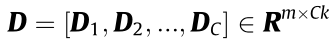, where C represents the number of modes, k represents the number of atoms of each mode, and D_C is a subdictionary of k atoms used to represent the characteristics of the Cth mode. The sparse matrix (S) of raw samples matrix (X) over D is S =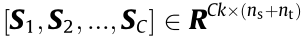, where  represents the sparse coding of Cth mode source domain data and represents the sparse coding of Cth mode target domain data. For the sake of simplicity, we record the sparse coding of  over D as =, where  is the coding coefficient of over the sub-dictionary D_C , is a matrix composed of the ith mode samples , which is a submatrix of X.

In order to improve the representation ability of the multimode data, prior constraints should be incorporated into the dictionary learning. First, the data should be well reconstructed by a dictionary and the corresponding sparse matrix; that is, X ≈ DS. Second, the data should be well represented by its own sub-dictionary and sub-sparse matrix ; that is, . Third, since the data can be well represented by its own subdictionary and sub-sparse matrix, the item should be as close to zero as possible, so the Eq. (1) can be transformed into the following formation [31]:

where d_b represents bth atom of the dictionary D. S_in and S_out are the expressions about S, which are given as follows:

where is the ath sample of X.

In particular, 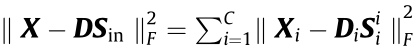 means that the data should be well represented by its own sub-dictionary and sub-sparse matrix .  That is, . Thus, the item  should be as close to zero as possible.

《3.2. Regularizations》

3.2. Regularizations

Since the source domain and target domain of the industrial system are affected by different environmental factors, the data distributions are different. To ensure that the learned dictionary captures the latent common mechanism information rather than irrelevant extrinsic interference in the source domain and target domain, a straightforward way is to reduce the distribution difference by minimizing some predefined metrics. MMD regularization is considered to be a nonparametric metric to express the distribution difference between domains [27], which can make the centers of the sparse matrices 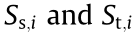close. Mathematically, the MMD regularization is expressed as follows:

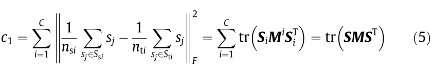
where c₁ represents the MMD regularization between the source domain and the target domain, represent the numbers of samples of ith mode in source domain and target domain, respectively, s_j is a sparse code in sparse matrix S, Mⁱ represents the ith mode part of MMD matrix M, which can be calculated as follows:

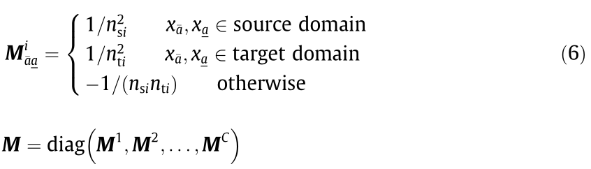
where  represents the element of  in the row and column,  is the   sample of X , and is the   sample of X.

It is well known that the distribution of observed data in the same mode should be the same. However, due to the uncertainty of the operating environment, the data in the same mode also exhibit certain differences. In order to eliminate the interference from the uncertain environment, it is preferable to make the sparse code of the same mode data become closer to each other no matter which domain the data comes from. That is, each column vector in should be close to each other. Thus, the value of  should be as small as possible,  where  is the center of .  Accordingly, the following constraint should be introduced.

where c₂ refers the intra-mode distances of all modes, and I is the identity matrix. The LDA-like matrix H can be obtained as follows:

where  is a vector with length  ,with all elements equal to 1,  is the total number of data for ith mode in the source domain and target domain. The regularization of Eq. (7) appears to be similar to the LDA regularization [34], so it will be called ‘‘LDA-like regularization” from this point on.

In summary, the MMD and LDA-like regularizations can be thought of as a progressive relationship. The MMD regularization makes the source domain center of each mode close to the target domain center of each mode. In a complementary way, the LDAlike regularization makes the data of the same mode closer to each other, in order to reduce the intra-mode distance. Based on the synergy effect of these two regularizations, the proposed method was formulated by joining Eqs. (2), (3), and (7) together; the objective function of the proposed method can be rewritten as follows:

where β₁ and β₂ (β₁, β₂ > 0) are hyper-parameters of the MMD regularization and the LDA-like regularization, respectively; and these hyper-parameters can balance the weight between the reconstruction error and the regularization constraints. Since the proposed method reduces the distribution divergence between the source domain and the target domain, it can achieve the effect of eliminating extrinsic environmental interference.

《3.3. Optimization》

3.3. Optimization

The optimization variables of the above objective function are D and S. Since the optimization problem is not a joint convex problem for both variables, but is separately convex to D (while holding S fixed) and convex to S (while holding D fixed), the alternative optimization method is introduced to calculated the optimal values of D and S iteratively [35].

3.3.1. Updating D

When updating the dictionary by fixing S, the objective function can be simplified to

After constructing a new data matrix and a new sparse matrix , , where O is the zero matrix of the same dimension as X, the objective function (Eq. (10)) becomes

The objective function can be solved effectively by using the Lagrange dual method [35]. First, consider the Lagrangian:

where L is Lagrange function,  is the introduced nonnegative parameter.

Minimizing the Lagrangian (Eq. (12)) by D yields the Lagrangian dual problem, as follows:

where B is the Lagrangian dual formula; is a diagonal matrix consisting of ,  = diag(). The Lagrangian dual problem (Eq. (13)) can be optimized by the Newton method or by a conjugate gradient. After maximizing B () , we obtain the optimal bases D as follows:

3.3.2. Updating S

The matrix S will be updated column by column. When s_j is being updated, the objective function can be expressed as follows:

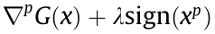
where Q, P, and h_j are intermediate variables in the simplification process of the objective functions. Q = diag (0,0,...,1,1,1,...,0,0,0), P = I – Q, and . Q is a diagonal matrix, and 1 is present only on the corresponding k positions of the mode of s_j . x_j is the jth sample in X.  is the pth element in s_j . We optimize Eq. (15) through a feature-sign search algorithm [27,35]. Define g (s_j) as follows:

where g (s_j) is the differentiable part of the Eq. (15). In order to address the feature-sign search algorithm for the problem in Eq. (15), a lemma should be introduced. 

Lemma 1: Define a continuous function over x as  ; the optimal necessary conditions of   are 

where   is a continuous differentiable function over vector x [36,35], is the pth element in vector x,  and  is the partial derivative of over  .

Proof: We provide a brief proof through a reduction to absurdity. Assume that there is an element in the optimal solution x that does not meet the condition. First, for ≠ 0, 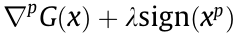≠ 0,  it is obvious that =≠ 0. Therefore, we can find another value  to take the place of  to make  be smaller. This is contradictory to the assumption. Second, for =0, , since  is a continuous differentiable function, we can find an  ＜0 to take the place of  and 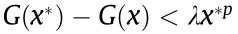is met. Therefore,  , which is also contradictory to the assumption. For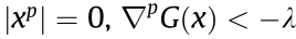, the same way can be used to show that the assumption is not true.

According to Lemma 1, the necessary condition in Eq. (15) can be described as follows:

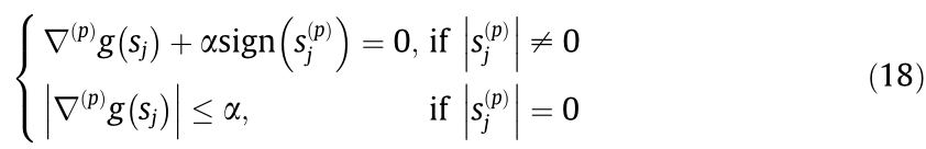
When the first condition is violated, The objective function  in Eq. (15) is differentiable over  because the sign of  is known, and it becomes an unconstrained optimization problem (QP). When the second condition is violated, assume that . Since  must be greater than zero, in order to minimize the local value of  must decrease. Since  starts at zero, any infinitesimal adjustment to  will make the sign of negative. Thus, we directly let the sign of  be –1. Then,  is similarly differentiable over  , and the problem can be solved simply. If  can be updated in the same way.

Accordingly, the complete process of the sparse matrix optimization algorithm is summarized as shown in Algorithm 1.

《3.4. Online process monitoring》

3.4. Online process monitoring

After the common dictionary D is obtained, the process monitoring and mode classification task will be carried out.

3.4.1. Process monitoring

Dictionary D and the orthogonal matching pursuit (OMP) algorithm [37] are used to calculate the sparse code s_j of the target domain data x_j in the training set; the reconstructed residual (RES) of the target domain data in the training set can be obtained according to Eq. (19).

where represents the L₂ norm of the vector, and r is the reconstruction error of sample x.

Next, the kernel density estimation (KDE) [38] is used to calculate the residual distribution interval of the data in the target domain, which can be used to detect whether the new testing data is normal or abnormal. When the new testing data x comes from the target domain, the sparse code s is obtained by using the same OMP algorithm; then RES r of the testing data can be obtained using Eq. (19). When the RES r belongs to the above distribution interval, it is normal data. Otherwise, it is faulty data.

3.4.2. Mode classification

After testing data is detected as normal data, mode classification is carried out, and the data x is identified by Eq. (20).

where sⁱ is sub-sparse code of s.

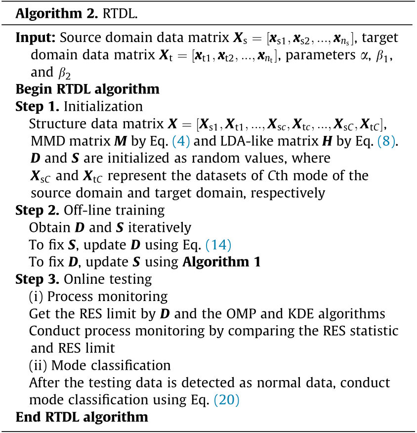
In summary, the complete model flow of the proposed method is summarized in Algorithm 2.

《4. Illustrative experiments》

4. Illustrative experiments

In this section, extensive experiments are carried out on a numerical simulation, the CSTH benchmark, and a wind turbine system to demonstrate the effectiveness and superiority of the proposed RTDL method. For the sake of performance visualization and parameter sensitivity analysis, the MMD regularization and LDAlike regularization are introduced separately in the numerical simulation in order to make it possible to visually observe the distribution of the samples. For the CSTH benchmark and the wind turbine system, the proposed method is compared with some state-of-theart methods for a performance comparison.

《4.1. Performance visualization and parameter sensitivity analysis》

4.1. Performance visualization and parameter sensitivity analysis

4.1.1. Datasets

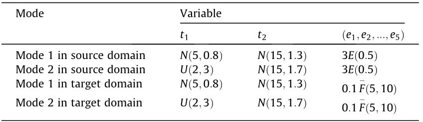
Experiments on a numerical simulation are performed to verify the motivation and intuitively evaluate the performance. The data generation model of the numerical simulation is as follows:

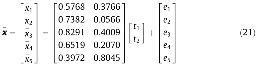
where  is the observed variable of process monitoring, t₁ and t₂ are two independent input variables of the data simulation model, and are the noise of the observed variable due to the current environment interference. For the sake of brevity, we assume that there are two modes in the source domain and target domain. The mode state is determined by the independent input variables t₁ and t₂ , while the environment interference   results in domains difference. A detailed description of the data is shown in Table 1, where  represents the Gaussian distribution whose mean is u and whose variance is  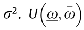denotes a uniform distribution that ranges from  to .  denotes an exponential distribution with the parameter    represents an F distribution with the degrees of freedom as . Abnormal data are collected from mode 2 in the target domain, with the bias faults occurring in x₂ .

For the training data, we collect 100 pieces of normal data for each mode in the source domain and 10 pieces of normal data for each mode in target domain. For the testing data, we collect 50 pieces of normal data for each mode and 300 pieces of abnormal data in the target domain.

《Table 1》

Table 1 Detailed description of data generation.

4.1.2. Performance visualization experiments

As mentioned above, MMD regularization and LDA-like regularization can eliminate distribution divergence from different perspectives. In order to verify that both have the ability to eliminate distribution divergence, we separately introduce one of them to observe the distribution of the samples visually by setting the other regularization parameter as zero. The training data are utilized to learn a common dictionary. Next, the sparse code of the source domain data, target domain data, and abnormal data are obtained through the common dictionary and OMP algorithm. We visualize the sparse code by means of PCA. The visualization is shown in Fig. 2.

Fig. 2(a) shows the raw data distribution. The domain distribution divergence that occurs is due to environmental interference. The abnormal information is obscure. Figs. 2(b) and (c) show that, with one of the regularizations used on its own, the distribution divergence is partly eliminated and the abnormal information emerges by means of dictionary learning. Fig. 2(d) shows that the source data and target data are completely mixed and the abnormal information can easily be identified by means of the proposed method using both regularizations. Accordingly, the experimental results agree with the motivation of this paper (Section 2.3).

《Fig. 2》

Fig. 2. Distribution of samples. (a) Raw data; (b) sparse code learned by dictionary learning with LDA-like regularization; (c) sparse code learned by dictionary learning with MMD regularization; (d) sparse code learned by dictionary learning with both regularizations.

4.1.3. Parameter sensitivity analysis experiments

The parameter α is an important adjusting parameter in dictionary learning that controls the sparsity of S. In general, α can be selected by observing the sparsity of S, which represents the percentage of nonzero elements in matrix S. As shown in Fig. 3, a satisfactory process-monitoring result can be obtained when the sparsity rate (SPR) ranges from 20% to 50% approximately; thus, the parameter sensitivity analysis for SPR verified the robustness of the proposed method.

《Fig. 3》

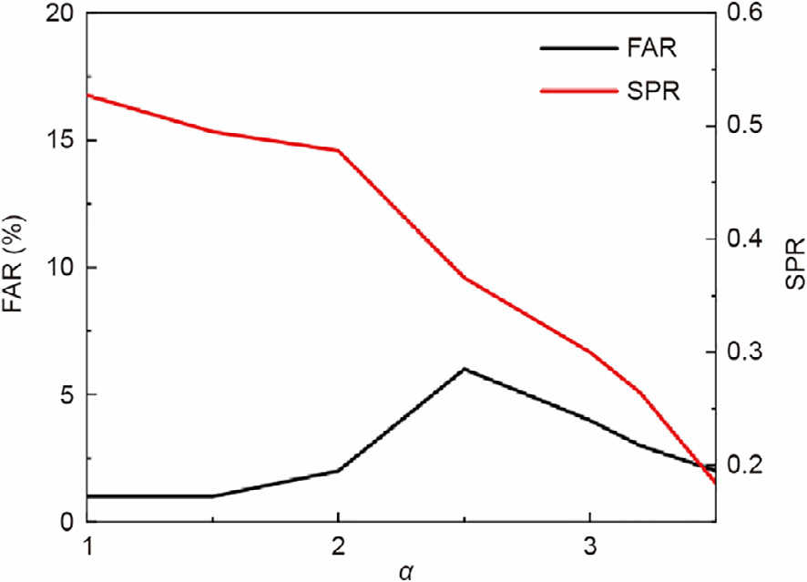
Fig. 3. Sensitivity analysis of the RTDL for FAR and SPR with parameter α. FAR: false alarm rate.

Next, the process-monitoring performance is shown for the modified β₁ and β₂ parameters. Let β₁ change from 10¹ to 10⁵ , while β₂ changes from 10 to 70. The false alarm rate (FAR) and fault detection rate (FDR) are considered to be two evaluation indexes for process monitoring. The results are shown in Figs. 4 and 5. It can be seen that the FAR is always lower than 3% and the FDR is always greater than 80% when β₁ and β₂ are changed. This performance of the process monitoring is commendable, even though β₁ and β₂ are changed in a wide range. When the values of β₁ and β₂ are too small, the learned dictionary can reconstruct the training data well; however, the irrelevant environmental interference of the training data is also learned by the dictionary. When the values of β₁ and β₂ are too big, the objective function is only to reduce the distribution difference between the domains; the learned dictionary cannot reconstruct the process data well, and underlying semantic information such as the mechanism information from the data will be lost. Both of these cases reduce the ability of the dictionary to capture the common latent information in the process data, resulting in a poor performance in process monitoring. In order to choose a suitable value for these hyper-parameters, an optimization method such as the grid search can be selected.

《Fig. 4》

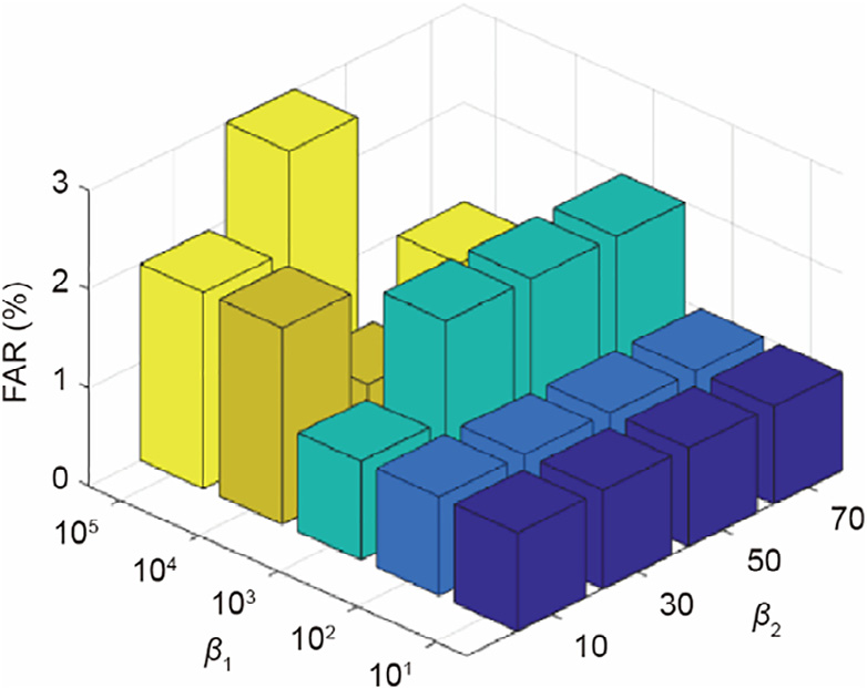
Fig. 4. Sensitivity analysis of the RTDL for FAR with parameters β₁ and β₂.

《Fig. 5》

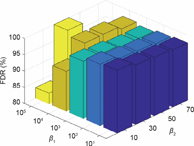
Fig. 5. Sensitivity analysis of the RTDL for FDR with parameters β₁ and β₂.

《4.2. Performance comparison experiments》

4.2. Performance comparison experiments

4.2.1. Datasets

Since the performance of the proposed method is commendable in the numerical simulation, we will now consider its performance in realistic industrial scenarios. Two datasets were prepared for these experiments.

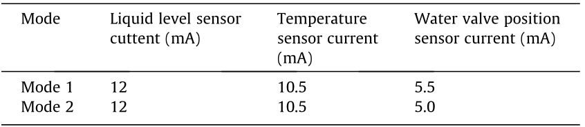
(1) CSTH: The CSTH process is a nonlinear real platform that has been widely used as a benchmark for evaluating different process-monitoring methods [39]. The principle of CSTH is shown in Fig. 6. In the CSTH process, there are two physical balances: a mass balance and a thermal balance. Cold water and hot water simultaneously flow into the sink, are stirred, and are heated by steam [40]. Suppose that this process has two modes, where the mode state is determined by the liquid level setting, temperature setting, and hot water valve position setting. The details are given in Table 2. To simulate environmental interference, we add an exponential distribution variable E(0.5) to all observed variables in order to form the source domain and an F distribution variable 0.1 to all observed variables in order to form the target domain. An additivity fault is imposed onto the observed flow variable to generate abnormal data. We collect 100 data for each mode in the source domain and 30 normal data for each mode in the target domain in order to form training data. The testing data consist of 50 data for each mode and 200 abnormal data in the target domain.

《Fig. 6》

Fig. 6. CSTH schematic diagram. TC: temperature controller; FC: flow controller; LC: liquid level controller; TT: temperature sensor; FT: flow sensor; LT: liquid level sensor; sp: set point. Reproduced from Ref. [40] with permission of Elsevier, ©2008.

《Table 2》

Table 2 The sensor current signal setting parameters of CSTH.

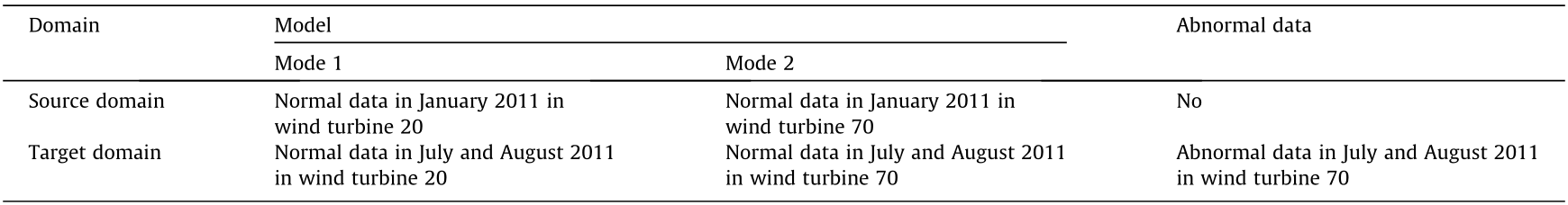
(2) Wind turbine system: The data on the wind turbine system come from a wind power company in Beijing. The data were sampled every minute from 1 January 2011 to 11 November 2011 by eight wind turbines, and the 15-dimensional data shown in Table 3 were used for process monitoring and mode classification. There are different manifold structures among the data of each wind turbine, which can be considered to be the operating modes of the wind turbine system. The temperature and wind in summer are different from those in winter, resulting in different operating temperatures and operating powers for the wind turbine, and leading to data distribution divergence. The wind turbine system is affected by different environmental interferences in different seasons. We assume the winter season to be the source domain while the summer season is the target domain. A detailed description is shown in Table 4. The training data is composed of 350 normal pieces of data for each mode in the source domain and 50 normal pieces of data for each mode in the target domain. A number of 50 normal pieces of data for each mode and 300 abnormal pieces of data in the target domain are taken to constitute the testing data. Due to the huge difference in the dimensions of the wind turbine system data, all the data were normalized before the experiment.

《Table 3》

Table 3 Features used in the wind turbine system experiment.

《Table 4》

Table 4 Detailed description of the wind turbine system data.

4.2.2. Comparison experiments for process monitoring

In order to evaluate the proposed method quantitatively, two other novel dictionary learning methods and an adaptive monitoring method are used for comparison. In addition, two data-processing strategies mentioned in Section 2.3 are used. Comparison methods include: label consistent K-singular value decomposition (LC-KSVD)(S+T), LC-KSVD(T), Fisher discrimination dictionary learning (FDDL)(S+T), FDDL(T), moving window PCA (MWPCA), and RTDL.

The LC-KSVD [41], FDDL [31], and MWPCA [42] methods are three state-of-the-art methods for process monitoring. LC-KSVD and FDDL possess the ability of mode classification, while MWPCA is another adaptive method for process monitoring. Here, LC-KSVD(S+T) and FDDL(S+T) refer to the LC-KSVD method and FDDL method, respectively, using all the source domain training data and target domain training data directly as the input data points without considering the different characteristics between the domains. LC-KSVD(T) and FDDL(T) refer to the LC-KSVD method and FDDL method, respectively, only using the target domain training data as the input data points. The MWPCA method uses all the source domain training data and the target domain training data directly as input data points without considering the different characteristics between domains. RTDL uses the source domain training data and the target domain training data discriminately as the input data points. In order to make the comparison fair, the size of the dictionary and other parameters are set to be the same. In order to compare the performance of the models, we refer to two indexes: FAR and FDR.

The results are shown in Figs. 7 and 8. As shown in these figures, the proposed method outperforms the baselines in terms of accuracy in both of the realistic datasets. There are also some interesting results. In CSTH, the FDR of LC-KSVD(S+T) is close to the FDR of LC-KSVD(T), but the FAR of LC-KSVD(S+T) is clearly greater than the FAR of LC-KSVD(T). This result agrees with the observation that if the distribution divergence of the domains is ignored, the model may easily confuse inter-domain difference information with abnormal information, leading to a poorer process-monitoring result.

《Fig. 7》

Fig. 7. Process-monitoring results of baselines and the proposed method on CSTH. (a) The DRE statistic of LC-KSVD(S+T); (b) the DRE statistic of LC-KSVD(T); (c) the DRE statistic of FDDL(S+T); (d) the DRE statistic of FDDL(T); (e) the T² statistic of MWPCA; and (f) the DRE statistic of RTDL. DRE: dictionary reconstruction error.

《Fig. 8》

Fig. 8. Process monitoring results of the baselines and the proposed method on the wind turbine system. (a) The DRE statistic of LC-KSVD(S+T); (b) the DRE statistic of LCKSVD(T); (c) the DRE statistic of FDDL(S+T); (d) the DRE statistic of FDDL(T); (e) the T² statistic of MWPCA; and (f) the DRE statistic of RTDL.

4.2.3. Comparison experiments for mode classification

The proposed method can deal with multimode data. In addition, when data is detected to be normal data, mode classification can be carried out; thus, in this section, the effectiveness of the mode classification is evaluated by a comparison with the baselines. Like the parameters setting, baselines can be used as the comparison experiment for process monitoring. Note that the mode classification task cannot be carried out by the MWPCA method, so that method is not utilized for the mode classification experiment. In order to compare the performance of the models, we refer to two indexes: mode 1 accuracy and mode 2 accuracy. The result is shown in Table 5. It can be seen that the performance of the proposed method in mode classification is better than that of the baselines, which further verifies the effectiveness of the proposed method.

《Table 5》

Table 5 Mode classification result.

《5. Conclusions》

5. Conclusions

Since industrial processes are often affected by a changeable operating environment, online monitoring data and historical training data do not always follow the same distribution. As a result, learned process-monitoring models based on historical training data cannot carry out the task of monitoring the online streaming data accurately. In this paper, an RTDL method was proposed. The proposed method is a synergy framework of representative learning and domain adaptive transfer learning. That is, the dictionary learning method, which projects the raw data into a subspace, is first used to learn a common dictionary to represent both the source domain data and the target domain data. After reducing the inter-domain distribution distance and the intramode distance in the subspace, the distribution divergence caused by environmental interference is eliminated, which improves the ability of the learned dictionary to represent internal semantic information, such as mechanism information. Through extensive experiments including a numerical simulation, the CSTH benchmark platform, and a real wind turbine system, the superiority of the proposed method for the domain transfer problem was demonstrated. Thus, it can be concluded that the proposed method can transfer knowledge from a single source domain to a single target domain. Since industrial processes usually encounter several operating environments, future works will focus on realizing knowledge transfer from multiple source domains to multiple target domains.

《Acknowledgements》

Acknowledgements

This work was supported in part by the National Natural Science Foundation of China (61988101) and in part by the National Key R&D Program of China (2018YFB1701100).

《Compliance with ethics guidelines》

Compliance with ethics guidelines

Chunhua Yang, Huiping Liang, Keke Huang, Yonggang Li, and Weihua Gui declare that they have no conflict of interest or financial conflicts to disclose.