
《1. Introduction》
1. Introduction
Black carbon (BC) or soot is mainly emitted due to the incomplete combustion of fossil fuels, biofuels, biomass, and other sources. BC is considered the largest anthropogenic climate forcer in the atmosphere after carbon dioxide (CO2). In contrast to CO2, BC is a short-lived pollutant, but the surface temperature response of snow and ice to a unit of BC radiative forcing is two to four times greater than that to a unit of CO2 radiative forcing [1]. Recently, it has been reported that BC is transported worldwide to areas such as the Himalayas and Tibetan Plateau, causing the rapid retreat of the glaciers in these areas with effects comparable to those of greenhouse gases [2,3]. However, large uncertainties remain in current estimates of the BC radiative effects, and one of the important reasons is that the BC resulting from various combustion sources exhibits different fractal dimensions during the BC aggregation process, leading to distinct radiative properties [4,5]. Road transport is a considerable source of anthropogenic BC emissions in urban areas [6]. A recent study has reported that the atmospheric BC concentrations near highways are higher than those in the residential and industrial areas of cities based on a largescale and high-density BC sensor monitoring network [7]. The radiative climate effect of BC and surge in vehicle population in cities (e.g., the metropolitan areas in China) prompted us to characterize on-road vehicle BC emissions.
The population of light-duty passenger vehicles (LDPVs) reportedly exceeded 200 million in China [8,9]. Over the past decade, the BC emissions from LDPVs have primarily been measured through laboratory tailpipe testing (i.e., dynamometer measurement) and ambient sampling methods (e.g., plume chasing and roadside and tunnel sampling). However, there are challenges in the accurate measurement of the BC emissions from LDPVs. In laboratory dynamometer testing, poor execution of the test cycles, for example, the New European Driving Cycle (NEDC), may induce a potential uncertainty in the results [10]. In remote sensing measurements, a short test duration of a few seconds or minutes may not adequately reflect the impact of complex traffic conditions. It may be insufficient to characterize BC emissions during the cold-start phase, which account for 18%–76% of the total BC emissions under the NEDC [11]. Compared to the above methods, portable emissions measurement system (PEMS) testing accurately records instantaneous pollutant emissions, vehicle driving parameters (e.g., vehicle acceleration and speed), and engine conditions (e.g., load and throttle position) through an onboard diagnostics (OBD) system. Hence, Europe and China have incorporated the PEMS method into the regulatory test protocols of their latest emission standards (i.e., Euro 6 and China 6, respectively) as the new Real-Driving Emissions (RDE) test [12,13]. Unfortunately, regulations have typically focused on gaseous pollutant and particle number (PN) emissions [13,14]. To date, except for Wang et al. [15], who reported real-time BC emissions based on an in situ method, no study has reported real-time BC emissions from onroad LDPVs. We note that compared to the more accurate tailpipe methods, BC emissions may be greatly overestimated under the ambient sampling methods. For example, Zheng et al. [11] measured the BC emissions from gasoline LDPVs using dynamometer tests and reported that the fuel-based emission factors (EFs) ranged from 1.7 to 8.9 mg·kg–1 , while the results of studies based on ambient remote sensing were much higher (e.g., ~75 mg·kg–1 reported by Liggio et al. [14] and 280 mg·kg–1 reported by Jezˇek et al. [16]). Wang et al. [15] conducted a synchronization test and found that the BC emissions from the same LDPV were approximately ten times higher using the plume chasing method than those determined using the onboard tailpipe method (i.e., 313.0 mg·kg–1 versus 39.5 mg·kg–1 ). However, Wang et al. [15] did not simultaneously measure the operating conditions in real time and thus were not able to analyze their impacts on the BC emissions. The real-time measurement of BC emissions under different operating conditions based on the tailpipe method (e.g., the PEMS method) is critical to characterize the BC emissions from on-road LDPVs, but such analysis is missing in existing studies. Moreover, to our knowledge, no study has yet characterized the cold-start BC emissions from on-road LDPVs, while cold-start limits for gaseous pollutants have already been adopted in the Euro 3 and China 3 emission standards. Because of the large population of LDPVs, it is necessary to measure and characterize BC emissions, including the cold-start emissions, from LDPVs under real-world conditions.
In this study, instantaneous vehicle BC emissions were measured using a PEMS platform. Ten in-use LDPVs, including port fuel injection (PFI) engine vehicles and gasoline direction injection (GDI) engine vehicles, were selected in Shenzhen and Beijing, China. An AVL MSS Plus instrument (AVL List GmbH, Austria) was adopted to measure the instantaneous BC emissions related to micro-operation conditions. An in-depth analysis of the impacts of the engine technology, cold-start events, ambient temperature, and real-world driving conditions was conducted.
《2. Methodology》
2. Methodology
《2.1. The PEMS platform》
2.1. The PEMS platform
The PEMS platform (Fig. 1) in this study consists of a 2 in (1 in = 2.54 cm) exhaust flowmeter with an integrated Global Positioning System (GPS) module, Ecostar ambient-temperature humidity sensors (Sensor Inc., USA), a Ecostar gaseous analyzer (Sensor Inc.), a Ecostar PN detector (Sensor Inc.), and a BC detector with an MSS Plus integrated two-stage dilution system. The Ecostar sensors are compliant with the US Environmental Protection Agency (EPA)’s CFR40 part 1065 [17,18], and they record the vehicle exhaust volume and instantaneous speed, while the second-by-second gaseous emissions are measured, including CO2, carbon monoxide (CO), and total hydrocarbons (THCs), using the nondispersive infrared (NDIR) and flame ionization detector (FID) methods. The PN detector complies with the particulate measurement program (PMP) methodology and records the instantaneous PN concentration (with a size larger than 23 nm) via butanol condensation [13,19]. The exhaust gas passes through the exhaust flowmeter, and some of the exhaust gas and PN emissions are sampled and analyzed by the Ecostar sensors. In parallel, a portion of the exhaust is sampled by the AVL MSS Plus instrument, and the BC detector complies with the US Society of Automotive Engineer (SAE)’s AIR6142 standard for the accurate, reliable, and second-by-second measurement of nonvolatile particle emissions, operating based on the photoacoustic measurement principle [20]. The AVL MSS Plus instrument contains a built-in dilution system with a dilution ratio of 20 times and performs air filtration to maintain clean air after the dilution step. When air containing BC enters the laser measuring cavity of the AVL MSS Plus instrument, BC particles absorb the energy emitted by the laser and release a signal, which may be regarded as a sound wave, to be measured with microphones. Compared to light-absorbing methods such as the aethalometer, the AVL MSS Plus instrument overcomes the problem whereby the aethalometer underestimates the BC concentration by ignoring the effect of particle light scattering [21].
《Fig. 1》
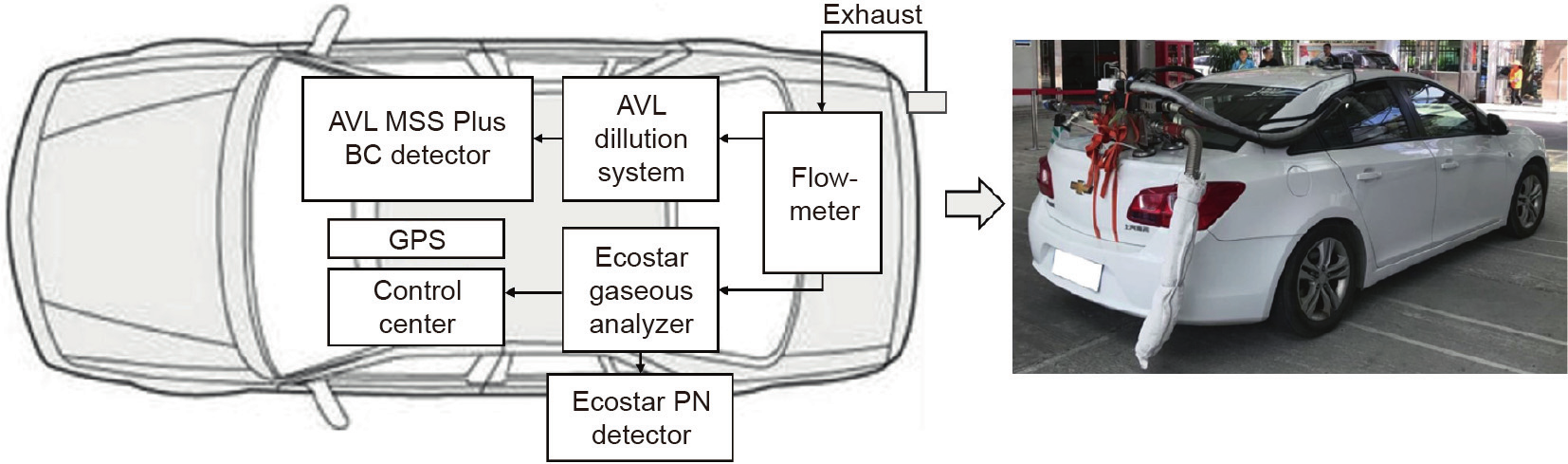
Fig. 1. PEMS platform in this study. GPS: Global Positioning System.
《2.2. Tested vehicles and sampling routes》
2.2. Tested vehicles and sampling routes
PEMS testing was conducted in 2019 in Shenzhen (summer) and Beijing (winter), China. A total of ten in-use LDPVs were selected for the measurements. The vehicles were manufactured from 2012 to 2018, and they complied with the China 4 (six vehicles) and China 5 (four vehicles) emission standards. Detailed information on the tested LDPVs is provided in Table 1. The China 4 emission standard was implemented in 2011 for PFI engine vehicles and in 2014 for GDI engine vehicles across China. The China 5 emission standard was implemented in eleven eastern provinces in 2016. By 2018, the vehicles complying with the China 4 and China 5 emission standards accounted for more than 80% of the registered LDPVs in China, representing the current trend of the LDPV market [22]. Among the selected LDPVs, six vehicles (#1–#6) had PFI engines, and four vehicles (#7–#10) relied on GDI engines. None of the LDPVs contained installed gasoline particle filters (GPFs). To study the BC emissions during cold start, all vehicles were soaked for longer than six hours before testing. It should be noted that in the Shenzhen (summer) test, soaking was conducted outdoors, and the difference between the inside-engine (i.e., engine oil) and ambient-temperatures was within 2 °C. In the Beijing (winter) test, the installation of the PEMS platform and vehicle soaking occurred in the laboratory. The laboratory temperature was approximately 25 °C, which does not reflect the cold-start emissions at low temperatures.
《Table 1》
Table 1 Summary of vehicle informations.

TWC: three-way catalyst.
a The model year could be one year earlier than the actual year of production and registration.
The testing routes included three road types: urban roads, rural roads, and motorways. The distances of each road type were approximately 16 km, and the average speeds on the urban roads, rural roads, and motorways were (21 ± 7), (50 ± 15), and (76 ± 14) km·h–1 , respectively (please refer to Table S1 in Appendix A). The test fuel complied with the China 6 gasoline standard and was directly acquired from gas stations [23].
《2.3. Emission calculations》
2.3. Emission calculations
The BC EFs can be calculated with Eqs. (1) and (2).

where EFBC,dis is the distance-based BC EF (mg·km–1 ), BCi is the BC concentration at second i (mg·m–3 ), DRi is the dilution ratio at second i, Vi is the exhaust volume at second i (m3 ·s–1 ), Si is the distance traveled by the vehicle at second i (km), EFBC,fuel is the fuel consumption-based BC EF (mg·kg–1 ), CO2i is the emission mass of CO2 at second i (g), COi is the emission mass of CO at second i (g), THCi is the emission mass of THCs at second i (g), wc is the carbon mass fraction in the gasoline (0.866), i is the starting time of the test, and n is the end time of the test. The EFs of CO2, CO, and THCs over the entire trip are listed in Table S2 in Appendix A.
The operating mode binning method is a useful methodology employed in modern vehicle emission models [24,25]. This method correlates the second-by-second vehicle emissions to the instantaneous driving conditions through a proxy parameter, defined as the vehicle specific power (VSP) [26,27]. The VSP was introduced by Jiménez-Palacios [28] to represent the real-time power demand of each vehicle. The VSP of the LDPVs is calculated according to Eq. (3) [29,30].

where VSPi is the vehicle specific power (kW·t–1 ) at second i, vi is the vehicle speed at second i (m·s–1 ), ai is the acceleration at second i (m·s–2 ), and θ is the road grade (radian). The roads in Shenzhen and Beijing, China are generally relatively flat. Therefore, the road grade is set to zero in this study. According to Zhang et al. [29], the operating mode bins were separated by the VSP and velocity, and the definitions of the operating mode bins are listed in Table S3 in Appendix A.
The average BC or PN emission rates based on the different engine technologies (i.e., PFI and GDI engines) and operating modes of each sample are calculated with Eqs. (4) and (5), respectively.
where ERj,i is the BC or PN emission rate under engine technology j at second i (mg·s–1 or s–1 , respectively),  is the average BC or PN emission rate under engine technology j and operating mode k (mg·s–1 or s–1 , respectively), Tk is the number of instantaneous data points under operating mode k, j is the type of the engine technology (e.g. PFI, GDI), and k is serial number of operating mode (defined by VSP and velocity).
To analyze the impact of the operating conditions, the BC emissions under special driving cycles, for example, the worldwide harmonized light-duty vehicle test cycle (WLTC) and NEDC, are calculated with Eq. (6).

where BCmass,l are the BC mass emissions under cycle l (i.e., the NEDC or WLTC) (mg);  are the average BC mass emissions under cold-start conditions, as measured in this study (mg);
  is the average emission rate under operating mode k (mg·s–1 ); and Tk is the duration of operating mode bin k under the given cycle. The speed profiles and time distributions of the various operating modes under the WLTC and NEDC are shown in Fig. S1 and listed in Table S4 in Appendix A.
The average speed in different phases of WLTC were 18.9 (low speed), 39.5 (medium speed), and 71.3 km·h–1 (high and extrahigh speed), which are comparable to the average speeds on the three road types in the present study. The maximum speed (131 km·h–1 ) covered all speed ranges in the present study. Hence, the WLTC was adopted as the baseline traffic pattern to harmonize the results of the different real-world tests. The BC EFs of each vehicle were normalized to the WLTC, as expressed in Eq. (7).

where EFBC,dis0 is the BC EF normalized to a typical traffic pattern (i.e., the WLTC) (mg·km–1 ), Pk is the time fraction of operating mode bin k under the WLTC, and  is the average speed during the WLTC (km·h–1 ).
In previous studies, we developed analytical functions of vehicle emissions and fuel consumption versus the average speed [29,31]. With the use of a similar method, we separated all test trips into microtrips and constructed a relationship between the relative BC emissions and average vehicle speed for all microtrips [27], as defined in Eq. (8).

where REFBC,m is the relative BC EF of the tested vehicles for microtrip m, EFBC,dis,m is the BC EF for microtrip m (mg·km–1 ), and m is the serial number of microtrip.
《3. Results and discussion》
3. Results and discussion
《3.1. BC emissions of the tested vehicles》
3.1. BC emissions of the tested vehicles
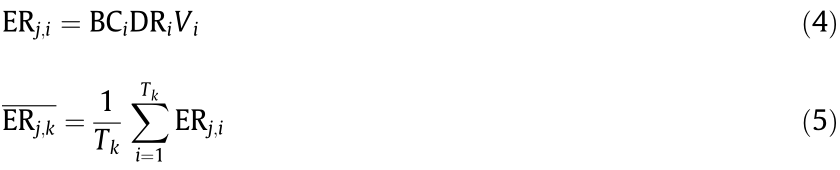
Compared to the PFI engine vehicles, the BC emissions from the GDI engine vehicles were much higher (Fig. 2). The average (distance-based) EF of the PFI engine vehicles (#1–#6) was (0.12 ± 0.06) mg·km–1 . In regard to vehicles #7–#10, the LDPVs with GDI engines, the BC emissions ranged from 1.10 to 1.56 mg·km–1 with an average of (1.31 ± 0.21) mg·km–1 , which are more than ten times higher than those from the PFI engine vehicles. The discrepancy in BC emissions between the PFI and GDI engine vehicles may occur due to the differences in fuel injection technology and mixture preparation [32–35]. In the GDI engine vehicles, the nonhomogeneous fuel/air mixture and wetting cylinder wall effect resulted in higher particulate (i.e., BC) emissions than those from the PFI engine vehicles.
《Fig. 2》
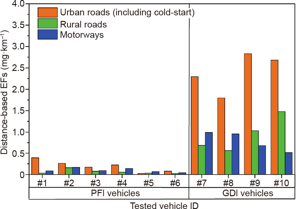
Fig. 2. BC emissions from each vehicle on urban and rural roads and motorways. ID: identity document.
Moreover, the trend of the average (fuel consumption-based) BC EF between the GDI and PFI engine vehicles was similar: (1.83 ± 1.01)mg·kg–1 for the PFI engine vehicles and (19.75 ± 4.39) mg·kg–1 for the GDI engine vehicles. The fuel consumption-based BC EFs were calculated based on the gaseous (i.e., CO2, CO, and THC) emissions (please refer to Table S2 in Appendix A). The EFs were (210.06 ± 38.64) g·km–1 for CO2, (0.91 ± 1.00) g·km–1 for CO, and (0.02 ± 0.01) g·km–1 for THCs. We found that the CO and THC emissions were much lower than those from the LDPV fleet (2.39–39.28 g·km–1 for CO and 0.11–3.30 g·km–1 for THCs) in earlier years (1998–2002) in China [36], which is attributed to the continuous tightening of the emission standards. In regard to the CO2 emissions, our results compare reasonably well to the results reported in previous studies [29,37,38].
《Fig. 3》

Fig. 3. On-road average BC emission rates under the different operating modes of the PFI and GDI engine vehicles.
When comparing the emission rates across the two engine technologies, we observed that the GDI engine vehicles produced higher BC emissions than did the PFI engine vehicles in all speed ranges (Fig. 3). Specifically, the BC emission rates of the GDI engine vehicles were (8.1 ± 1.6) times higher under the low-speed modes, (6.2 ± 1.0) times higher under the medium-speed modes, and (4.9 ± 1.1) times higher under the high-speed modes than those of the PFI engine vehicles. With the further penetration of GDI engine vehicles in China’s gasoline vehicle market, we recommend adopting BC emission control techniques as soon as possible. Chan et al. [39] reported that GPFs reduced the BC emissions from GDI engines by 73%–88% at 22 °C based on dynamometer tests. However, McCaffery et al. [40] found that the removal efficiency of GPFs was only 44% using the PEMS method for a GDI engine vehicle in Los Angeles, USA. Therefore, there may be a gap in the actual removal efficiency of the GPF for on-road GDI engine vehicles, and more tests are needed to accurately estimate the efficiency of the GPF. In addition, in all speed ranges, the average BC emission rate increased with the VSP. For instance, in bins 35–3Y (i.e., the high-speed operating modes), the average BC emission rates of the GDI engine vehicles increased from (0.009 ± 0.003) mg·s–1 in bin 35 to (0.04 ± 0.01) mg·s–1 in bin 3Y. Similarly, the average BC emission rate of the GDI engine vehicles increased eight-fold from bins 21 to 2Y (i.e., the medium-speed modes). In regard to the PFI engine vehicles, the average BC emission rates under the highspeed and high-VSP modes were a factor of 3 and 10, respectively, higher than those under the low-speed and medium-VSP modes, respectively.
We further examined the impact of the ambient temperature in the tests during the different seasons. However, since soaking in winter was carried out in the laboratory, the results only reflect the BC emissions at room temperature (~25 °C) under cold-start conditions and at low temperature ((3 ± 1)°C) under hot-running conditions. The BC EF of the China 4 PFI engine vehicles (#1 and #4) in winter was (0.150 ± 0.022) mg·km–1 , which is comparable to the vehicle emissions in summer (#2 and #3, (0.150 ± 0.078) mg·km–1 ). In contrast to previous studies, we observed relatively small differences between winter and summer [39,41]. We speculate that the ambient temperature imposes little effect on the hotrunning conditions but imposes a major effect on the cold-start conditions of LDPVs. Fig. S2 in Appendix A shows the on-road average BC emission rates of the tested vehicles during hot running in the different seasons. There is no significant difference (p > 0.05, where p is the value of probability) in BC emissions between the various ambient temperatures for both the PFI and GDI engine vehicles, which confirms our supposition. This observation is in line with previous laboratory measurements. As reported by He et al. [41], the average BC emissions under the hot-start WLTC were (0.16 ± 0.05) mg·km–1 at 30 °C and (0.59 ± 0.18) mg·km–1 at 7 °C for two PFI engine vehicles, and (1.14 ± 0.98) mg·km–1 and (0.66 ± 0.30) mg·km–1 , respectively, for two GDI engine vehicles, indicating no significant difference in BC emissions between the different ambient temperatures [41].
《3.2. Impact of the cold start on the black carbon emissions》
3.2. Impact of the cold start on the black carbon emissions
Based on the instantaneous BC measurements throughout the trips, we easily found that during the vehicle start-up phase (i.e., the cold start), the BC emissions are much higher than those on the hot-running urban roads (excluding cold-start emissions), which is consistent with the findings of a number of dynamometer studies reporting particularly high cold-start BC mass emissions [11,41,42]. For example, in Chan et al. [39], the BC EFs under Federal Test Procedure (FTP)-75 phase 1 (including a cold start) were nearly ten times higher than those under phase 3. Zheng et al. [11] reported that the duration of the cold start is shorter than 100 s (six samples) based on instantaneous BC measurements in dynamometer tests. Hence, we adopted a duration of 100 s to calculate the BC mass emissions under the cold-start events. The data indicated that the average mass EF of the PFI engine vehicles was (5.7 ± 0.6) mg during the cold start. Regarding the GDI engine vehicles, the average mass emissions of the cold-start vehicles were (16.1 ± 0.9) mg. Cold pistons and cylinder walls in GDI engines reduce fuel evaporation and increase fuel impingement, which produces more BC during fuel ignition [43]. In terms of the PFI engine vehicles, during the cold start, to compensate for the low volatility of gasoline, wall wetting and incomplete fuel vaporization result in high BC emissions [42].
The results indicate that the BC mass emissions during the cold start from the PFI engine vehicles account for 2%–25% of the total BC mass emissions. For the GDI engine vehicles, the cold-start BC mass emissions account for 22%–33% of the total BC mass emissions. The contributions of the cold-start BC emissions in this study are lower than those in other dynamometer tests [39,44]. For example, the BC mass contributions of PFI engine vehicles during the cold-start phase were reported to reach (44% ± 26%) under the NEDC [44]. This mainly occurs due to the short mileage in the dynamometer test (10.9 km under the NEDC versus (48.3 ± 0.2) km in the PEMS test), which increases the contribution of cold-start emissions. Moreover, in this study, the proportions of the cold-start BC emissions in the total BC emissions are higher for the GDI engine vehicles than they are for the PFI engine vehicles, which indicates that the highly concentrated BC emissions during the cold-start phase should be of concern, especially for GDI engine vehicles. The limits of cold-start emissions for gaseous pollutants have been incorporated in the China 3 emission standard, and a series of strategies based on engine control techniques has been adopted to minimize cold-start emissions. For instance, calibration of the fuel injection timing and variable valve timing may suppress BC (or particulate matter) emissions. Moreover, BC emissions could be optimized by increasing the cold-start idle speed (1500–2000 revolutions per minute (rpm)), which allows the engine to rapidly warm up to reduce the cold-wall quenching phenomenon during the cold-start phase [45]. For both GDI and PFI engine vehicles, the engine speed leaps above 1500–1600 rpm and then drops to nearly 1000 rpm within seconds (please refer to Fig. S3 in Appendix A for an example of vehicles #3 and #9), which coincides with the period of high BC emissions during the cold-start phase. Therefore, more technologies (e.g., the GPF) should be implemented, especially in GDI engines [46,47].
《3.3. Impact of the driving conditions on the BC emissions》
3.3. Impact of the driving conditions on the BC emissions
The driving conditions notably influence the BC emissions from LDPVs. The BC emissions from the tested vehicles on the rural roads were (56% ± 34%) lower than those on the hot-running urban roads. Improving the operating conditions and increasing the vehicle speed in metropolises (e.g., Beijing and Shenzhen) above 20 km·h–1 could effectively reduce the BC emissions on a perkilometer basis (will be shown below).
However, high engine speeds and loads on motorways could result in high BC emissions from both PFI and GDI engine vehicles. The average BC motorway EF was (60% ± 78%) higher than the rural road result. This observation is consistent with previous studies using dynamometer tests. In He et al. [41], the BC emissions in the extrahigh-speed phase were (103% ± 78%) higher than those in the high-speed phase for GDI engine vehicles and (490% ± 265% ) higher for PFI engine vehicles, indicating that PFI engine vehicles are more sensitive to an aggressive driving behavior.
Fig. 4 shows the contribution of each driving condition (coldstart roads, hot-running urban roads, rural roads, and motorways) to the BC emissions throughout the trips. The largest contributor comprised the hot-running urban roads (37% ± 15%), followed by the motorways (27% ± 12%), rural roads (20% ± 8%), and coldstart roads (17% ± 10%). The cold-start phase is considered an important contributor to BC emissions because while it only corresponds to less than 0.1% of the testing route distance, the proportion of the cold-start BC emissions in the total BC emissions is much larger. Notably, these two phases (i.e., cold-start and hotrunning urban roads), together contribute more than half to the total BC emissions (54% ± 14%). Furthermore, we observed that the contribution of the motorways was higher for the PFI engine vehicles (31% ± 12%) than that for the GDI engine vehicles (20% ± 8%), which implies that the BC emissions from the PFI engine vehicles are more sensitive to high-load and high-speed conditions. The contribution of each driving condition to the BC emissions is highly associated with the selected routes. If we adopt average emission rates and Eq. (6) to calculate the BC emissions under the WLTC and NEDC, we find that the low-speed phase under the WLTC and the four Economic Commission of Europe (ECE) segments under the NEDC contribute 55% and 62%, respectively, of the total BC emissions for the GDI engine vehicles.
《Fig. 4》

Fig. 4. Contribution of each driving condition to the BC emissions from all tested vehicles.
Fig. 5 shows the correlation between the relative BC emissions and average vehicle speed in each traffic episode (the duration of the episode is about 300 s). The relative BC emissions notably increase when the average speed decreases below 20 km·h–1 when traffic congestion occurs. The relative BC emissions are less sensitive to the driving conditions at high speeds ranging from 30 to 80 km·h–1 . However, when the average speed exceeds 90 km·h–1 , the relative BC emissions increase with increasing average vehicle speed. We determined a nonlinear function y = 1/(0.00031x2+ 0:047x + 0:13) (where y is relative BC emissions, x is average vehicle speed) as the best fit between the relative BC emissions and average speed (R2 = 0.70).
《Fig. 5》

Fig. 5. Correlation between the average vehicle speed and relative BC emissions.
While we note that the adoption of GPFs could play a critical role in limiting the BC emissions from future LDPV fleets, improving the driving conditions could be an effective solution for the current in-use LDPVs to reduce BC emissions by avoiding BC emission-sensitive speed ranges under congested traffic conditions when the average vehicle speed is below 20 km·h–1 . For example, the relative BC emissions increase by 23% when the average vehicle speed decreases from 20 to 15 km·h–1 . Beijing has implemented a license control policy to control the vehicle population since 2011. Zhang et al. [29] estimated that the average speed of LDPVs will reach nearly 28 km·h–1 in 2020 under the license control scenario. In contrast, the vehicle population will exceed nine million in 2020 without the license control policy, and the average speed will decrease to 21 km·h–1 . The license control scenario results in 18% lower BC emissions than those under the no license control scenario. This highlights the importance of traffic congestion alleviation to mitigate BC emissions.
《3.4. Relationship between the real-world PN and BC emissions》
3.4. Relationship between the real-world PN and BC emissions
The real-world PN emission limit has been adopted in China and Europe as part of the China 6 and Euro 6 RDE tests, respectively, to detect the particle emissions from GDI engine vehicles or lowemission vehicles (i.e., GPF vehicles). Previous studies have reported a strong correlation between PN and BC emissions using the dynamometer method. Khalek et al. [48] reported a PN (60– 90 nm)-to-BC mass emission ratio ranging from 3.2 × 10¹² to 3.9 × 10¹² mg–1 for a GDI engine vehicle. In the study by Chan et al. [39], the PN-to-BC mass ratios ranged from 0.2 × 10¹² to 2 × 10¹² mg–1 [39]. In the present study, the real-world PN and BC emissions were jointly measured using the PEMS platform to explore the PN-to-BC mass ratios of the on-road LDPVs (#1, #3, #4, #5, #6, and #10). Fig. 6 shows the correlations between the average PN-to-BC emission ratios organized by the various operating bins. We observed a strong correlation between the BC and PN emissions (R2 = 0.90) with an average ratio of 1.8 × 10¹² mg–1 for all tested vehicles, which is consistent with previous studies. However, we found a more pronounced linear relationship between the PN and BC emissions for the GDI engine vehicles (R2 = 0.96) than that for the PFI engine vehicles (R2 = 0.76). We further compared the average ratios of the instantaneous PN-to-BC emission rates (ERPN/ERBC) according to the microscale operating conditions. We observed that the instantaneous ERPN/ERBC ratio of the GDI engine vehicles was less sensitive to the increase in VSPV in all speed regions than that of the PFI engine vehicles. For example, ERPN/ERBC ranged from 1.5 × 10¹² to 2.5 × 10¹² in the three speed ranges for the GDI engine vehicles. In contrast, from bins 11 to 3Y, ERPN/ERBC for the PFI engine vehicles increased from 8.8 × 10¹¹ to 4.0 × 10¹². This implies that caution should be exercised when using PN emissions to estimate the BC emissions from PFI engine vehicles since the ratios are highly associated with the instantaneous driving conditions.
《Fig. 6》

Fig. 6. (a) Correlations between the PN and BC emissions and (b) the average PN/BC ratios based on the operating mode.
《3.6. Comparison to previous studies》
3.6. Comparison to previous studies
Compared to other studies measuring tailpipe BC emissions using dynamometers or the PEMS method (please refer to Table 2 [11,14–16,39–42,49–55]), the BC EFs reported in the present study are in line with the reported results of various model year vehicles and driving cycles. For example, the BC emissions from PFI engine vehicles reported by Forestieri et al. [42] range from 0.06 to 2.20 mg·km–1 , which covers the highest and lowest emitters tested in the present study. The BC EFs of the GDI engine vehicles in this study are comparable to those reported by McCaffery et al. [40] and Forestieri et al. [42]. However, our results are lower than those reported by Zheng et al. [11] and Chan et al. [39], possibly because of the large displacement and high vehicle age in these two previous studies. Moreover, the distance of the testing routes in this study ((48.3 ± 0.2) km) is much longer than that in most dynamometer tests (e.g., 11 km under the NEDC), which leads to a small contribution of the cold start and therefore a low distancebased EF.
《Table 2》
Table 2 Comparison with previous studies.

Compared to other studies using different ambient sampling methods (please refer to Table 1), we found that tunnel or roadside studies may overestimate the BC EFs of LDPVs, even though the vehicles sampled in tunnel or roadside studies were operated without the impacts of a cold start [14,16,49–53]. For example, compared to the average fuel-based BC EF of (7.9 ± 8.8) mg·kg–1 in the present study, Liggio et al. [14] reported a median EF value of about 75 mg·kg–1 for gasoline LDPVs, and Park et al. [54] reported a range of 40–90 mg·kg–1 for LDPVs operating under different conditions, such as idling, acceleration and cruise. The average BC EF reported by Westerdahl et al. [55] using roadside monitoring was 300 mg·kg–1 , about 40 times higher than our results. The main reason for the overestimation of the BC EFs by the above tunnel or roadside studies lies in the difference in the measuring locations. The PEMS method samples the BC and CO2 concentrations at the tailpipe, which eliminates the disturbance of the BC and CO2 in the ambient air and increases the signal-to-noise ratio. In contrast, roadside or plume chasing is susceptible to the dispersion of BC and CO2 emissions from other vehicles. Wang et al. [15] found that the difference in BC concentration reached 37 μg·m–3 between the tailpipe and tailpipe background and 4 g·m–3 between the plume and ambient environment, while the difference in CO2 concentration was 15 200 and 36 ppm (1 ppm = 1 mg·m–3 ), respectively. Therefore, the ratio of the BC increment to the CO2 increment in the tailpipe is much higher than that in the plume, leading to a large uncertainty in the BC EFs determined with the roadside or plume chasing method. Wang et al. [15] further demonstrated that the BC EFs in pipe and plume chasing tests reached 39.5 and 313.0 mg·kg–1 , respectively, for the same LDPVs in a synchronization test. Furthermore, the background CO2 concentration is a key parameter in the chasing method and heavily affects the determined BC EFs. However, the background CO2 level surrounding the target vehicle in the chasing test is easily elevated by a high density of other vehicles on urban roads [55]. Jezˇek et al. [56] reported that BC EFs varied between –40% and 80% if the background CO2 level changed by ±1 standard deviation, which may result in a wide BC EF range [56]. Moreover, it is also possible that the vehicles tested in the present study are high-emission vehicles such as malfunctioning or high-mileage vehicles. High-emission vehicles could result in very high emissions in plume chasing and roadside studies. Zielinska et al. [57] reported that the particulate matter emissions from malfunctioning gasoline vehicles were approximately six times higher than those from well-functioning gasoline vehicles.
《4. Conclusions》
4. Conclusions
This study developed a PEMS platform to measure the realworld instantaneous BC emissions from six PFI engine LDPVs and four GDI engine LDPVs in China. Testing was conducted on various road types. The results revealed that the GDI engine vehicles produce significantly higher average BC EFs and instantaneous BC emissions than those produced by the PFI engine vehicles. This indicates that BC emission control technologies such as the GPF should be adopted as soon as possible, with increasing penetration of GDI engine vehicles in the Chinese gasoline vehicle market. Furthermore, we calculated the real-world BC emissions during coldstart events (the first 100 s). The results indicated that the coldstart BC emissions were (5.7 ± 0.6) and (16.1 ± 0.9) mg for the PFI and GDI engine vehicles, respectively, accounting for 2%–25% and 22%–33%, respectively, of the total BC emissions throughout the entire trip, while the cold-start duration of the vehicles was less than 0.1% of the total travel distance. This indicates that the highly concentrated BC emissions during the cold-start phase should be of concern, especially for GDI engine vehicles. The hot-running roads, rural roads, and motorways contributed (37% ± 15%), (20% ± 8%), and (27% ± 12%), respectively, to the total BC emissions. Moreover, a strong correlation was found between the average vehicle speed and relative BC emissions (R2 = 0.70). The BC emissions significantly increased under congested traffic conditions with an average speed below 20 km·h–1 . This highlights the importance of traffic congestion alleviation to mitigate BC emissions. The BC and PN emissions were linearly correlated (R2 = 0.90), and the instantaneous emission ERPN/ERBC ratios of the GDI engine vehicles were less sensitive to the increase in VSPV in all speed ranges than those of the PFI engine vehicles. This implies that caution should be exercised when adopting PN emissions to estimate the BC emissions from PFI engine vehicles since the above ratios are highly dependent on the instantaneous driving conditions.
《Acknowledgments》
Acknowledgments
This work was supported by the National Natural Science Foundation of China (51708327 and 51978404). The contents of this paper are the sole responsibility of the authors and do not necessarily reflect the official views of the sponsors.
《Compliance with ethics guidelines》
Compliance with ethics guidelines
Xuan Zheng, Liqiang He, Xiaoyi He, Shaojun Zhang, Yihuan Cao, Jiming Hao, and Ye Wu declare that they have no conflict of interest or financial conflicts to disclose.
《Appendix A. Supplementary data》
Appendix A. Supplementary data
Supplementary data to this article can be found online at https://doi.org/10.1016/j.eng.2020.11.009.


 京公网安备 11010502051620号


