Expanding the Scope of Multivariate Regression Approaches in Cross-Omics Research

Abstract

Recent technological advancements and developments have led to a dramatic increase in the amount of high-dimensional data and thus have increased the demand for proper and efficient multivariate regression methods. Numerous traditional multivariate approaches such as principal component analysis have been used broadly in various research areas, including investment analysis, image identification, and population genetic structure analysis. However, these common approaches have the limitations of ignoring the correlations between responses and a low variable selection efficiency. Therefore, in this article, we introduce the reduced rank regression method and its extensions, sparse reduced rank regression and subspace assisted regression with row sparsity, which hold potential to meet the above demands and thus improve the interpretability of regression models. We conducted a simulation study to evaluate their performance and compared them with several other variable selection methods. For different application scenarios, we also provide selection suggestions based on predictive ability and variable selection accuracy. Finally, to demonstrate the practical value of these methods in the field of microbiome research, we applied our chosen method to real population-level microbiome data, the results of which validated our method. Our method extensions provide valuable guidelines for future omics research, especially with respect to multivariate regression, and could pave the way for novel discoveries in microbiome and related research fields.

Content

《1. Introduction》

1. Introduction

Biology and medicine have long since entered the age of big data, accelerated by the development of analytical methods and diagnostic techniques in sequencing, proteomic analysis, metabolic analysis, and so forth. For example, next-generation sequencing in the last decade has made sequencing individual genomes and metagenomes feasible, even for single research laboratories, compared with the international efforts and years-long work on the Human Genome Project [1]. Microbiome research, which has also been accelerated by sequencing techniques [2], has revealed the importance of microbial communities in human health and diseases [3], among other fields. All these developments have produced an unprecedentedly large volume of data with high dimensionality, which in turn has promoted general research interest in multivariate regression analysis [4,5]. Multivariate regression aims to model the relationships between a set of responses and a set of features, in contrast to common regression, which usually depicts a one-to-one relationship [6,7]. Response variables (or dependent variables) are the outcomes of an experiment that researchers hope to explain, and predictor variables (or independent variables) are the controlled inputs that may cause the variation in the responses. For example, in a genomics study, the responses in such regressions could be human traits, and the features could be genetic or environmental factors. Therefore, multivariate regression can be applied in all aspects of our daily lives. For example, it is broadly used in economics to investigate the factors that influence stock returns [8]. It is also familiar and common in the field of biology [9]. For example, it is applied in clinical trials to help researchers explain the relationships between drug ingredients and pesticide effects [10]. Recently, in genomics research, including metagenomics research and in combination with metabolomics, proteomics, and so forth, multivariate regression has played a significant role in understanding the association and potential causation of important traits [11].

Various attempts have been made to use multivariate methods to address specific challenges. Principal component analysis (PCA) is one of the oldest and best-known eigenvector-based multivariate analysis techniques [12]. It is widely used to find a linear combination of variables that describe the most variance using orthogonal transformation when the number of variables is large. By projecting the data to a lower-dimensional space showing the dominant gradients, PCA can reveal the internal structure of data [13,14]. In practice, principal component regression (PCR) is a linear regression model that uses PCA to estimate the regression coefficient matrix. Canonical correspondence analysis (CCA) is another approach that is often used to explain the relationships between two sets of variables by reducing dimensionality [15]. It aims to find a linear combination that can describe the maximum correlations between predictor variables and responses. Another method often used to find the relations between two matrices is partial least-squares (PLS) regression [16]. It summarizes covariance structure by projecting the response variables and predictor variables into a new space to build a linear regression model. Although the above methods are widely used in studies, three main statistical problems arise. The first problem is that traditional methods often ignore the possible interrelations between the response variables of observational data. The second problem is that some of the approaches do not allow variable selection, which is essential in exploratory experiments when the number of predictor variables is large. Third, some real databases often have large total numbers of variables and small sample sizes, leading to unreliable solutions [17,18].

Based on these considerations, we analyzed a class of new methods (reduced rank regression (RRR) and its extension) that improve the interpretability of regression models by considering the correlations between responses [19,20]. RRR is a data reduction method similar to PCA that creates new variables to summarize a large amount of information in the original data [21]. In particular, it defines a set of linear combinations of predictor variables to best explain the total variance in the response variables, and has many desirable characteristics such as simplicity, computational efficiency, and outstanding predictive performance. When the number of predictor variables is large, the selection of important variables is another issue of interest to researchers. Although some traditional methods are available—such as random forest, which makes predictions by constructing a multitude of decision trees—they are more suitable for cases with a single response variable. Therefore, some RRR-based approaches have adopted the ideas of group selection methods such as the group least absolute shrinkage and selection operator (group lasso) method, which is used for variable selection when determining the group structure among variables. In nutritional epidemiology and genetics, many reports use RRR approaches; yet comprehensive analysis of the properties of different RRR-based approaches, as well as their applicability to real data—especially metagenomic-centered data—remains to be conducted [22–25]. Here, we used simulated data with different dimensionalities to compare the performance of various RRRbased approaches with that of other multivariate regression methods with similar properties, examined their strengths and limitations under different scenarios, and finally applied them to largescale public metagenomic datasets.

《2. Methods》

2. Methods

《2.1. Description of the approaches tested in this study》

2.1. Description of the approaches tested in this study

In this study, we used the basic multivariate linear regression method as the starting point, and then included a few RRR-based approaches and other multivariate regression approaches for comparison. For each method, the definition and rationale are explained below.

2.1.1. Multivariate linear regression

A multivariate linear regression model is composed of multiple predictor variables X₁, X₂, ..., X_p and multiple response variables Y₁, Y₂, ..., Y_q. Each response variable is represented by a linear regression of the predictors; that is,

where c_kj is the regression coefficient relating X_k to Y_j, and is the error term with mean zero.

In addition, this formula can be rewritten with n observations, as follows:

where X is an n × p predictor matrix, Y is an n × p response matrix, C is a p × q matrix of regression coefficients, and E is an n × q error matrix.

We estimate the coefficient matrix C based on the least squares criterion; that is

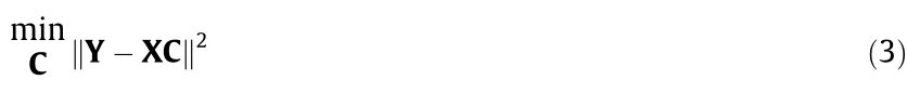
where denotes the Frobenius norm.

Using the ordinary least-squares (OLS) method, we obtain the estimate of C, , which is calculated as following:

2.1.2. Reduced rank regression

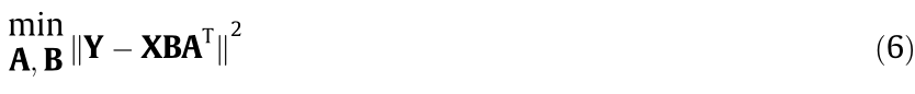
However, the OLS method provides a rough estimate since it ignores the possible interrelationships between response variables and simply performs a separate estimation for each response variable. Therefore, here, we introduce RRR, which constrains the rank of coefficient matrix C. We suppose C is of lower rank, r = ran(C) ≤ min(p, q), and C can be expressed as a product of two rank r matrices, C = BA^T , where B has p × r dimensions and A has q × r dimensions. The multivariate regression model (2) could be rewritten as

In addition, XB has n × r dimensions representing a set of r linear combinations of X, which can be interpreted as the latent factors driving the variation in Y. Therefore, RRR helps reduce the dimensionality of the predictor variables and improves computing efficiency.

We can rewrite the optimization function (3); that is

The set of solutions and is given as

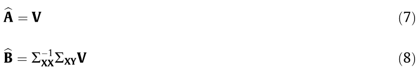
where 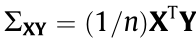, and V represents the eigenvectors of 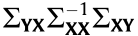corresponding to the eigenvalues, in which [26].

2.1.3. Sparse reduced rank regression (SRRR)

SRRR is an extensive RRR approach that focuses on not only dimensionality reduction, but also variable selection [26,27]. It imposes the sparsity of the coefficient matrix by adding a penalty to the least-squares estimation, and thus has unique properties. Compared with RRR, which uses all predictor variables to build the latent factors, SRRR can be used to select the useful ones from a large number of variables and exclude the redundant ones by introducing a group lasso penalty [28]. Therefore, the optimization formula (6) can be rewritten as follows:

where is the penalty parameter. The constraint A^TA = I is applied to satisfy the identifiability conditions, where I denotes the identity matrix. In addition, if is set to zero, the entire i-th row of matrix B will be zero, and the i-th predictor variable will be inactive.

By using the subgradient method or variational method, the optimization problem can be solved, but defining p penalty parameters () by cross-validation (CV) could be time consuming. To reduce the number of tuning parameters, two strategies are usually used [26]:

(1) Group lasso penalty: Set all values equal to .

(2) Adaptive weighting lasso penalty: Calculate each based on the original data structure as 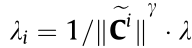, where is a root-n consistent estimator of C and is a positive integer [29].

2.1.4. Subspace assisted regression with row sparsity (SARRS)

SARRS also focuses on solving the issues of low rankness and sparsity in the coefficient matrix [30]. This new estimation scheme can be used in adaptive sparse reduced rank multivariate regression and achieves the goals of dimensionality reduction and variable selection. Furthermore, compared with SRRR as discussed above, SARRS improves performance when the number of predictor variables exceeds the sample size.

During the process of optimizing the regression with group sparsity, two penalty functions can be used:

(1) Group lasso penalty: , where is the penalty parameter and B is the parameter matrix to be optimized.

(2) Group minimax concave penalty (MCP): = 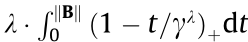, where is a positive integer greater than 1 and denotes its positive part, that is = [31].

2.1.5. Sparse partial least-squares regression (SPLS)

SPLS method is based on PLS and further encourages sparsity in the multidimensional direction in predictor space; thus, it achieves variable selection [17]. It first selects the predictor variables that have strong correlations with the responses, and then adds additional ones that have strong partial correlations. SPLS employs a different reduced rank structure than SRRR and does not directly focus on the prediction of the response variables, creating a possible weakness in its prediction.

2.1.6. Regularized multivariate regression for identifying master predictors (REmMap)

REmMap method is different from the above methods since it assumes not only that only some of the predictors are correlated with the responses, but also that these predictors may influence only some of the responses [32]. This is reasonable because in real situations, researchers often pay more attention to specific responses than to others. REmMap can fit multivariate regression models with high dimensionality and small sample sizes, and can introduce both overall sparsity and group sparsity into the coefficient matrix to detect master predictors.

2.1.7. Summary

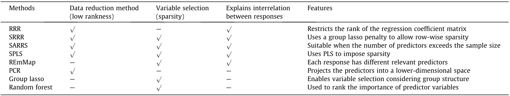
The characteristics of the methods discussed in this article are summarized in Table 1.

《Table 1》

Table 1 Methods comparison.

《2.2. Test of method performance based on simulated data》

2.2. Test of method performance based on simulated data

2.2.1. Simulation setups

To illustrate and compare the performance of SRRR, SARRS, SPLS, REmMap, and some traditional approaches (PCR, group lasso, and random forest), we first introduce a simulation study to generate data and analyze them using the above approaches. We use a similar simulation setup as Chen and Huang [26]. The central idea of the simulation study is to analyze some predictor variables that are correlated with the response variables and some that are uncorrelated. Then, we use these methods to examine which of them can most accurately determine the relationship and achieve good predictive performance.

We generate data with the multivariate linear equation Y = XBA^T + E. In this model, the n × p design matrix X follows a multivariate normal distribution , where has diagonal elements of 1 and off-diagonal elements of Matrix B and matrix A comprise the coefficient matrix of the model. In p × r matrix B, the first p₀rows follow N(0,1) , and the remaining p – p₀ rows are zero. The q × r matrix A is generated from N(0,1) . Matrix E is a random noise matrix defined by , where is the magnitude of the noise and has diagonal elements of 1 and off-diagonal elements of . Then, the n× q matrix Y is calculated from the above model.

We generate three sets of data including a training set, validation set, and test set. The training set is used to fit the models based on the various approaches. The validation set is used to tune the parameters inside the models and estimate the noise variance. Lastly, we use the data from the test set to evaluate the performance of the models we built.

To explore the methods’ applicability in different situations, we conduct the simulation study using several different cases. First, since it is sometimes difficult for researchers to obtain sufficient samples to carry out trials, we want to test the performance of the approaches when applied to both small sample sizes and large sample sizes. Second, we are also interested in the influence of the number of variables. Real data such as microbiological data and genetic data often include high-dimensional predictor variables or response variables. Based on the above considerations, we simulate six cases as follows, where n is the sample size of the data and p and q are the numbers of variables in X and Y, respectively.

Case 1: Small sample size, n < p

Case 1a: n = 20; p = 100; q = 25

Case 1b: n = 20; p = 25; q = 25

Case 1c: n = 20; p = 25; q = 100

Case 2: Large sample size, n > p

Case 2a: n = 200; p = 100; q = 25

Case 2b: n = 200; p = 25; q = 25

Case 2c: n = 200; p = 25; q = 100

The simulation procedure and the methods discussed are coded in R using the spls, rrpack, remMap, pls, glmnet, and randomForest packages; the code for the SARRS method was provided by the authors of the respective packages. The computational procedure has been specified and listed in Appendix A.

2.2.2. Evaluation of various methods

In each case, we repeat the simulation procedure 500 times and use the following metrics to measure and compare the performance of the above multivariate regression methods:

(1) Mean square error (MSE): The MSE is used to show the predictive accuracy of these methods, and is defined as follows:

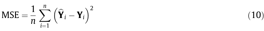
where is the predicted value of .

(2) R squared: The R² index is the proportion of the variance in the response variables that can be explained by the predictor variables. It is often used to describe how well a model fits data. A larger R² indicates a better goodness of fit for the model.

(3) Theil inequality coefficient (TIC): The TIC is another indicator used to reflect the difference between the fitted values and the true values. It is defined as follows:

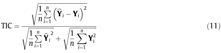
The TIC ranges from zero to one, and a smaller TIC indicates a higher prediction accuracy.

(4) Sensitivity (TPR) and specificity (SPC): TPR and SPC are commonly used to evaluate the accuracy of variable selection. TPR is the ability to select the true relevant variables and is calculated as the ratio of the number of correct selections with respect to the total number of correlated input variables. SPC is the ability to select the true irrelevant variables and is calculated as the ratio of the number of correct selections with respect to the total number of uncorrelated input variables. A method that has both high TPR and high SPC means can select the relevant variables accurately.

(5) Area under the curve (AUC): The AUC is also used to measure the rate of correctly selecting the true relevant variables [33].

(6) Overall rating: The overall rating index is calculated by using the above evaluation metrics. The method with better performance has a higher overall score.

《2.3. Application to real population-level microbiome data》

2.3. Application to real population-level microbiome data

To illustrate the practicality of the above methods for realworld problems, we apply them to data from the Belgian Flemish Gut Flora Project (FGFP; discovery cohort: n = 1106) from the work of Falony et al. [34]. This research is aimed at discovering the relationships between microbiota variation and environmental factors such as host features, geography, and medication intake. Sixty-six clinical and questionnaire-based variables are discussed as possible predictors, with 74 microbiome species as responses after selection.

We conducted CV to randomly split the data into a training set and a test set. A model was built to fit the data, and its performance was evaluated by the above metrics. We repeated the process 50 times to examine the stability of variable selection.

《3. Results》

3. Results

《3.1. Simulation study reveals the distinct properties of each method》

3.1. Simulation study reveals the distinct properties of each method

In the simulation, we applied SRRR (with the group lasso penalty and adaptive weighting group lasso penalty), SARRS (with the group lasso penalty and group MCP penalty), SPLS, REmMap, PCR, group lasso, and random forest to the different cases and used CV to tune the low-rankness parameters for each approach. Their overall performance is shown in Fig. 1.

《Fig. 1》

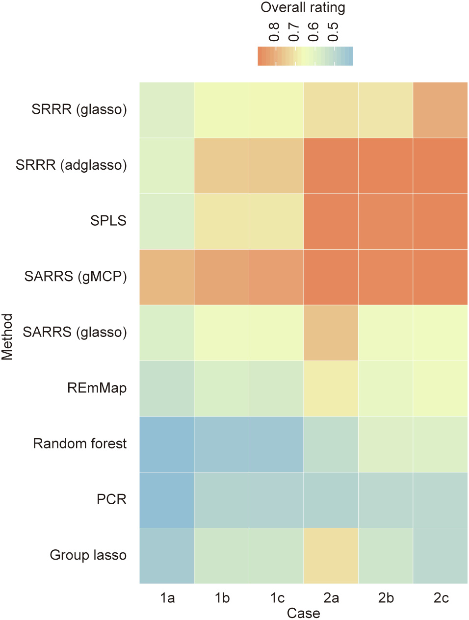
Fig. 1. Overall evaluation of all methods, shown as a heatmap. The x-axis denotes the different cases, and the y-axis denotes the methods. The color of each cell represents the corresponding overall rating. A higher overall rating indicates better performance. glasso: group lasso penalty; adglasso: adaptive weighting group lasso penalty; gMCP: group MCP penalty.

The heat map shows that all the methods perform worse in case 1 than in case 2, which is consistent with our prediction. In addition, it is clear that SARRS (with the group MCP penalty) best fits all the cases and, when the sample size becomes larger, SRRR (with the adaptive weighting group lasso penalty) and SPLS are also applicable and perform equally well.

The performance of each method is measured by the criteria detailed above, and the result for case 1 is shown in Fig. 2.

《Fig. 2》

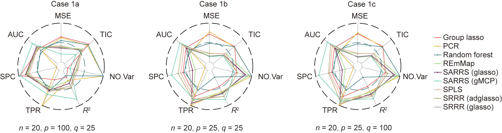
Fig. 2. Performance evaluation of all methods for cases 1a, 1b, and 1c, shown as a radar plot. The center of the circle indicates 0. For R² , TIC, TPR, SPC, and AUC, the edge of the circle indicates 1. Therefore, if a method has a high R² , TPR, SPC, and AUC, and a low TIC and MSE of the response matrix, we conclude that this method has good performance. The NO.Var index gives the number of variables selected with each method, where the center of circle indicates 0 and the edge indicates the number of predictor variables.

In case 1a, we have an extremely small sample size, and the number of predictor variables is greater than that with the small size; therefore, most methods do not have good predictive and variable selection performance. Except for PCR, which could not select the relevant variables, the methods’ SPCs are approximately 0.75, and their TPRs are approximately 0.55, indicating under selection. However, compared with the traditional methods (PCR, group lasso, and random forest), the new approaches discussed in this article all perform better, especially the SARRS method with the group MCP penalty. This method has the lowest MSE and TIC as well as the highest R² , SPC, and AUC. This outcome is consistent with the discussion in the methodology section, which specifically noted that SARRS is the most suitable and accurate method when the number of predictor variables is much larger than the sample size.

In cases 1b and 1c, the number of predictor variables and the sample size become closer. We find that all the models fit the simulated data better than in case 1a due to the higher R² and the lower TIC. The plot also shows the superiority of SRRR in terms of prediction accuracy, since SPLS and REmMap have larger MSEs than SRRR and SARRS. Furthermore, regarding variable selection, we can see that SARRS (with the group MCP penalty), SRRR (with the adaptive weighting group lasso penalty), and SPLS have better performance, with much higher SPCs, than the others, indicating a balance in selecting the true relevant variables and avoiding overselection.

In case 2, we explore a situation with a large sample size; it is obvious that all methods have better performance than in case 1, as shown in Fig. 3.

《Fig. 3》

Fig. 3. Performance evaluation of all methods for cases 2a, 2b, and 2c, shown as a radar plot. The center of the circle indicates 0. For R² , TIC, TPR, SPC, and AUC, the edge of the circle indicates 1. Therefore, if a method has a high R² , TPR, SPC, and AUC, and a low TIC and MSE of the response matrix, we conclude that this method has good performance. The NO.Var index gives the number of variables selected with each method, where the center of circle indicates 0 and the edge indicates the number of predictor variables.

We first discuss case 2a, in which there are many more predictor variables than response variables. Regarding predictive performance, the new methods that we are interested in all have an extremely low MSE for the coefficient matrix, even approaching 0, an average TIC of approximately 0.27, and an average R² of approximately 0.72, indicating a good model fit. Furthermore, the traditional methods still behave poorly in this aspect. Regarding variable selection, all methods have higher TPRs and AUCs than in case 1. SARRS (with the group MCP penalty), SRRR (with the adaptive weighting group lasso penalty), and SPLS also have extremely high SPCs, indicating that they could accurately select all of the relevant variables and reject all of the irrelevant variables.

In case 2b, we reduce the number of predictor variables to be the same as the number of response variables, thereby increasing the difference between the sample size and the number of variables. Under this circumstance, all the new methods perform well in terms of prediction. However, in variable selection, the outcomes of the methods are polarized. The best method is still SRRR (with the adaptive weighting group lasso penalty), followed by SARRS (with the group MCP penalty) and SPLS, whose selection accuracies approach 1. However, for the other methods, the SPC is generally low, indicating an overselection problem. As case 1c is similar to case 1b, case 2c is also similar to case 2b. However, compared with cases 1b and 1c, the increase in the sample size causes cases 2b and 2c to display much better performance in terms of both prediction accuracy and variable selection.

《3.2. Application to real population-level microbiome data》

3.2. Application to real population-level microbiome data

The data characteristics of the case study, in which the sample size (n = 1106) is far greater than the number of variables (p = 66; q = 74), are consistent with case 2b in the above simulation study. Based on the former discussion, we know that the most suitable method to apply for this dataset is SRRR (with the adaptive weighting group lasso penalty). Therefore, we build an SRRR model to analyze the relationships between the environmental indexes and bacterial composition, and discuss the predictive accuracy and variable selection outcomes. The results are shown in Fig. 4.

《Fig. 4》

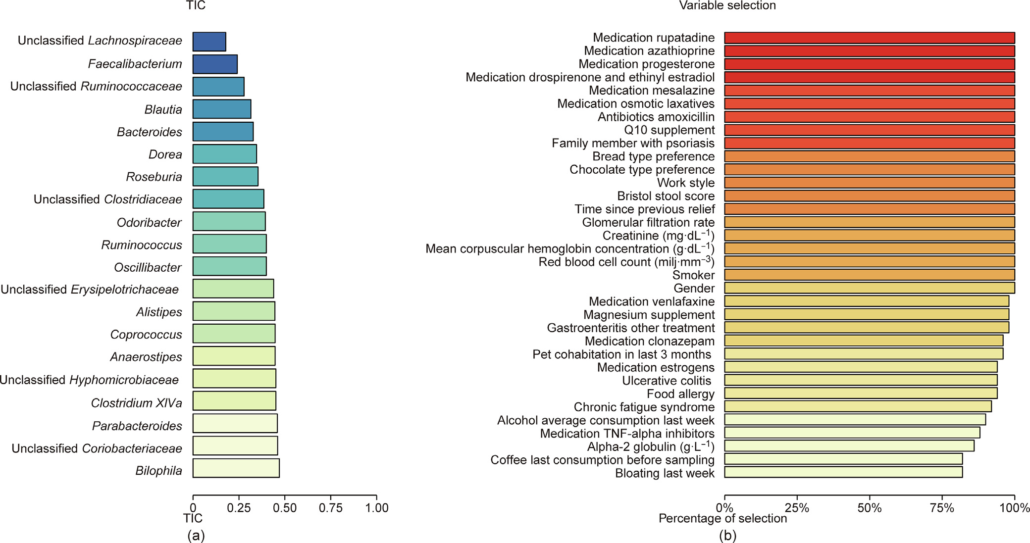
Fig. 4. Performance evaluation of the SRRR (with the adaptive weighting group lasso penalty) for real population-level microbiome data. (a) A bar plot using the TIC index to demonstrate the predictive performance of the SRRR model for each response variable. We display the 20 variables with the lowest TICs in this plot. (b) A plot showing the percentage of selection in 50 cross-validations for each predictor variable.

The average TIC of the model is 0.56, which is higher than the 0.26 for case 2b in the simulation study. However, since we know that the real data are noisier than the simulated data, we conclude that this TIC is acceptable but not convincing in terms of adequate model prediction. However, upon a closer examination of each response variable, we find that the variables with a low TIC are those reported in many previous studies, including the FGFP [34], such as Faecalibacterium (with a TIC of 0.24), Blautia (0.32), Bacteroides (0.33), Roseburia (0.35), and Ruminococcus (0.40). These are key butyric-producing bacteria that are involved in many diseases when they are at a low abundance, as low butyrate production by the microbiome leads to a higher level of inflammation and metabolic disorders [35,36]. Therefore, these variables were explained well by the predictors selected by SRRR and could be predicted by the coefficient matrix calculated by SRRR.

Finally, we examined the robustness of the variable selection. Since we repeated the CV procedure 50 times, the predictor variables that were selected in more than 80% of the cases are the most meaningful. Fig. 4(b) shows the 34 variables that were selected most frequently, including gender, smoker, red blood cell count (RBC), creatinine, stool score, mean corpuscular hemoglobin concentration (MCHC), and many kinds of medications. This outcome is consistent with the importance of the effects of medications, as discussed in a previous study [37].

《4. Conclusion》

4. Conclusion

As the volume and dimensionality of data increase in nearly every field of research, biomedical research will continue to be one of the most important and fast-developing areas. When extracting the maximum value from data, obtaining correct, useful, and meaningful associations between different measures or omics levels poses an important challenge [38]. Here, we examined some representative methods, including extensions of RRR and other multivariate regression methods, and used both simulated data and real microbiome-centered data to address the strengths and limitations of these methods, which might be instructive for future applications to microbiome and other related omics data.

We included a total of nine method–parameter combinations, including seven methods; furthermore, for two of them, two different penalties were used. We simulated data with different sample sizes/dimensionalities and compared the predictor and response variables with/without large differences in dimensionality. From the results when comparing case 1 and case 2, the importance of a large sample size became clear, which could greatly improve the performance of all methods. In particular, compared with case 1, SPLS has much better predictive accuracy in case 2, indicating that it is more applicable when the sample size is large. Under a situation similar to case 1, when the sample size is small, the best method is SARRS with a group MCP penalty, which has outstanding performance in terms of both prediction and variable selection. When the sample size is large, as in case 2, SARRS (with the group MCP penalty), SRRR (with the adaptive weighting group lasso penalty), and SPLS all perform very well; upon closer examination, SRRR (with the adaptive weighting group lasso penalty) performs slightly better than the other two methods.

We used this information to select the best method for a real scenario: namely, the published FGFP data, for which microbiome data and the environmental factors identified in the study are available. With roughly similar dimensionalities for the two types of variables, we decided to use SRRR with the adaptive weighting group lasso penalty. First, we identified the bacterial groups that are best explained by the environmental changes. The identified bacterial groups confirm previous assertions that the butyrate-producing bacteria are of great importance in human health and may serve as a link to those environmental factors. In addition, since environmental factors were considered to be predictors (i.e., features selected to be associated with bacterial groups), we also managed to replicate the most important features in the published study, again demonstrating the reliability and robustness of the selected method.

Researchers should carefully choose a proper penalty when fitting models. For example, in the SRRR method, when n > p, the adaptive weighting group lasso penalty improves both the prediction accuracy and variable selection. When n < p, the adaptive weighting results in a lower TPR but higher SPC than those for the unweighted group lasso penalty. This could be explained by the fact that when we introduced weighting to the SRRR calculation procedure, the variables that were filtered out earlier had larger weights for their penalty terms and were no longer included in the model. Therefore, SRRR with an unweighted penalty will select more variables and lead to a high SPC.

In conclusion, we examined the applicability of several multivariate regression approaches and tested their performance under different omics scenarios, which in reality may differ vastly in their sample sizes and dimensionalities. Based on this, we were able to recommend the best method. Admittedly, our preliminary analysis could not be further expanded at this stage to incorporate the phylogenetic information between different measures (e.g., species) in many omics data, since this would require priori information regarding the connectedness and similarity between those measures. We also used a renowned microbiome dataset to show that our method of choice can largely recapitulate the findings obtained by single-variate analysis and improve the consideration between variables and combined feature selection. These findings will facilitate the choice of methods in future, larger scale omics research, including microbiome-centered studies.

《Acknowledgments》

Acknowledgments

This project was supported by the National Key Research and Development Program of China (2018YFC2000500), the Strategic Priority Research Program of the Chinese Academy of Sciences (XDB29020000), the National Natural Science Foundation of China (31771481 and 91857101), and the Key Research Program of the Chinese Academy of Sciences (KFZD-SW-219), ‘‘China Microbiome Initiative.”

《Compliance with ethics guidelines》

Compliance with ethics guidelines

Xiaoxi Hu, Yue Ma, Yakun Xu, Peiyao Zhao, and Jun Wang declare that they have no conflict of interest or financial conflicts to disclose.

《Appendix A. Supplementary data》

Appendix A. Supplementary data

Supplementary data to this article can be found online at https://doi.org/10.1016/j.eng.2020.05.028.

Show More