

《1. Introduction》
1. Introduction
Brain electrical activity—that is, the excitement of neurons—is an important reflection of brain function [1–7]. Continuously observing the electrophysiological signals in the brain is important for understanding the function and message-processing mechanisms of the nervous system [8–20]. The electrical response of the brain to stimulation has been well studied in isolated areas of the cortex or in a small number of neurons (e.g., the evoked cortex potential (ECP), which can be recorded by a multi-electrode matrixes); however, little is known of the exact temporal–spatial progress of the brain’s reaction to peripheral nerve stimulation. This is a critical knowledge gap, because brain function is accomplished by the coordination of numerous neurons and nuclei. Such complicated process cannot be well understood with the fragmental information on the nervous system obtained by traditional methods. However, determining the functional parameters of the brain as completely as possible is extremely challenging, given the shortcomings of traditional ECP-recording methods based on a single electrode or multi-electrode matrix [21–23]. First, recorded signals only reflect the action potential of a few cortical neurons around the electrode [24,25]. Therefore, it is difficult to obtain the electrophysiological characteristics of whole cell populations in the target regions and analyze complicated brain functions. Second, a slight change in electrode position results in a major fluctuation in the signals as well as significant individual variations, which makes it easy to miss the common regularities. Third, traditional craniotomy and placing electrodes onto the surface of the cortex or into the cortex result in severe trauma and extensive disturbance to the brain. Moreover, it is difficult to achieve long-term, continuous observation using traditional methods. Therefore, grasping the dynamic temporal–spatial progress of the brain in response to the stimulation of peripheral nerves can be extremely useful in obtaining a deeper understanding of the working patterns of the brain.
In this research, we develop a novel electrophysiological method with an orthogonal lead system and mini-invasive procedures, and investigate the overall excitation progress in different brain functional regions corresponding to peripheral stimulations in rats. We also provide a fully typical ECP atlas of different peripheral nerves and their subdivided branches, making it possible to visualize the temporal–spatial properties and interactions of the brain and peripheral nerve reconstructions.
《2. Methods》
2. Methods
《2.1. Description of animals and ethics statement》
2.1. Description of animals and ethics statement
Adult male Sprague–Dawley rats weighing 200–250 g were acquired from the Laboratory Animal Center of Peking University People’s Hospital (PKUPH; specific pathogen free level, animal use permit No. SYXK (jing) 2011-0010). The rats were maintained on a 12 h light/dark cycle with free access to pellet food and water. The anesthetic, surgical, and postoperative care protocols used in this research conformed to the National Institutes of Health guidelines regarding animal experimentation and were approved by the Research Ethics Committee at PKUPH. Every effort was made to minimize animal suffering and reduce the number of animals used.
《2.2. Surgical procedures and electrode implantation》
2.2. Surgical procedures and electrode implantation
Rats were randomly separated into groups to test the ECPs of the median, ulnar, and radial nerves and branches separately. For the three main forearm nerve trunks, 18 animals were used to obtain the electrical signals (six animals for one nerve). For the branches of the three nerve trunks, another 18 animals were used to obtain data and avoid unnecessary reaction errors in the rats due to different operation planes and a long operation time.
The rats were anesthetized using sodium pentobarbital with a dosage of 30 mg·kg-1 via intraperitoneal injection; they were also given 15 mg·kg-1 sodium pentobarbital to maintain the depth of the anesthesia when necessary. The head and right limbs were shaved and sterilized. The trunks and subdivided branches of the median, ulnar, and radial nerves were exposed from the surrounding tissues and moistened by infiltration with saline gauze. The room temperature was maintained at 20–25 °C while the experiment was performed. A homeothermic blanket system was used to maintain the rectal temperature at 37.0–37.5 °C and to prevent hypothermia, which may affect the physiological activity of the brain.
The rat head was fixed in a stereotaxic instrument. An approximately 3 cm long midline incision was made. After adequate exposure of the operation region from the lambda to the bregma, 3% hydrogen peroxide was used to clean the skull surface. As reported by Khazipov et al. [26] and Paxinos et al. [27], the electrode positions A1, A2, B1, and B2 were identified (Figs. 1(a) and (b)). Ag/AgCl pins (head size of 8 mm, wall thickness of 0.2 mm, inner diameter of 0.5 mm, tail length of 1 mm, and diameter of 0.5 mm) were used as recording electrodes and were inserted into the marked points on the skull surface (diameter of 0.5 mm and depth of 1 mm) (Figs. 1(b) and (c)). Our method skillfully avoided the location of sinusoids in order to reduce the possibility of accidental injury of the blood sinus causing intracranial hematoma.
《Fig. 1》
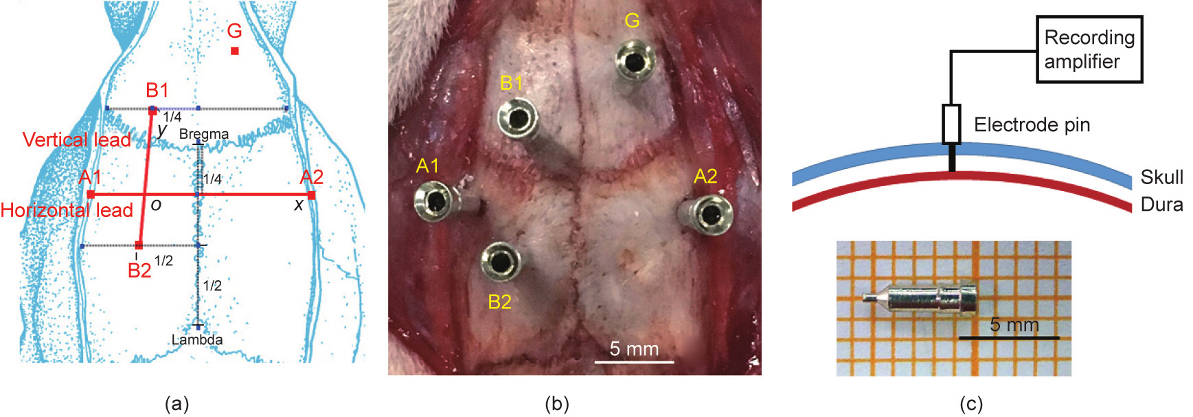
Fig. 1. (a) Using the bregma and lambda as references to determine the electrode positions at A1, A2, B1, and B2. The horizontal lead is the line connecting A1 and A2; the vertical lead is the line connecting B1 and B2. (b) Orthogonal lead system in rat. (c) Pins were used as the recording electrodes. The electrodes are just broken through the skull diploe and are exposed to the dura; the cerebral cortex still remains intact. G is the ground point.
《2.3. Evoked cortex potentials recording》
2.3. Evoked cortex potentials recording
The target nerve and its branches were carefully exposed. An electrical stimulator (MedlecSynergy; Oxford Instrument Inc., UK) was set to the designed position using bipolar electrodes. Spherical Ag/AgCl electrodes were used to collect the cortical signals. The line connecting A1 to A2 was set as the horizontal (H) lead, while the line connecting B1 to B2 was set as the vertical (V) lead. The stimulus intensity was 0.09 mA, the duration was 0.2 ms, and the repetition rate was 5 pulse per second (pps). A monophasic square-wave constant current pattern (3 Hz, 100 μs pulse width) was used. On average, 300 sweeps were used for the acquisition of one ECP trace. To illustrate the waveform of the ECP, we marked the negative wave as N, and the positive wave as P. If the amplitude was higher than 10 μV, the waveform was marked as N or P. Otherwise, the waveform was marked as n or p. ECPs were recorded by stimulating the median, ulnar, and radial nerves and their subdivided branches, respectively.
《2.4. Temporal–spatial parameters conversion from an orthogonal lead system》
2.4. Temporal–spatial parameters conversion from an orthogonal lead system
In a rectangular coordinate system, the positive direction of the horizontal ECP vector x points from A1 to A2, while the positive direction of the vertical ECP vector y points from B2 to B1. The resultant ECP vector ρ is synthesized by the horizontal and vertical components. To better understand the temporal–spatial character of the ECP, we converted the rectangular coordinate system into a polar coordinate system, where point o was the intersection of vector x and vector y, ρ =  and θ = tan-1(x, y) , which was intersection angle from ox to ρ. Time (t) was set as another parameter in the polar coordinate system. Thus, ECP = (ρ, θ,t).
《2.5. Median nerve transection model》
2.5. Median nerve transection model
A total of six rats were anesthetized with 30 mg·kg-1 of pentobarbital sodium by intraperitoneal injection. The operation sites were shaved and sterilized, followed by decortication. After being exposed, the median nerve was transected at 3 mm above the cubital fossa. The proximal stump of the median nerve was ligated with 5-0 nylon sutures and stitched to the adjacent muscle in the reverse direction to prevent nerve growth. The wound was rinsed with sufficient saline and then closed with 5-0 nylon sutures. The rats were placed back into the cages. Electrophysiological examinations were performed four months after the operation to assess the change in ECP.
《2.6. Data analysis》
2.6. Data analysis
Data in this work are expressed as the mean ± standard deviation (SD). Analysis and statistics were performed using SPSS 20.0 software (SPSS Inc., USA).
《3. Results》
3. Results
《3.1. The position relationship between the electrode and the cortical functional areas in rat》
3.1. The position relationship between the electrode and the cortical functional areas in rat
In this experiment, the orthogonal lead was located above the somatic motor and the somatosensory region in the left brain. The green and red areas in Fig. 2 represent the somatic motor and the somatosensory area, respectively; the H lead and V lead orthogonally cross through the corresponding cortical functional areas.
《Fig. 2》

Fig. 2. Relationship between the orthogonal lead and the cortical functional areas. A schematic diagram of the functional areas in the rat cortex. The green and red areas represent the somatic motor and the somatosensory area, respectively. S1FL: primary somatosensory cortex forelimb region; S1HL: primary somatosensory cortex hindlimb region; M1: primary motor cortex; M2: secondary motor cortex.
《3.2. Temporal–spatial characteristics of ECPs induced by the median nerve and its subdivided branches》
3.2. Temporal–spatial characteristics of ECPs induced by the median nerve and its subdivided branches
Stable ECPs can be obtained in both the H lead and the V lead by stimulating the median nerve trunk. The latency of the ECP in the H and V leads was (1.21 ± 0.04) and (1.25 ± 0.06) ms, respectively, which was in accordance with the time required for the nerve pulse to spread from the stimulated site to the cortex (Fig. 3 and Table 1).
《Fig. 3》
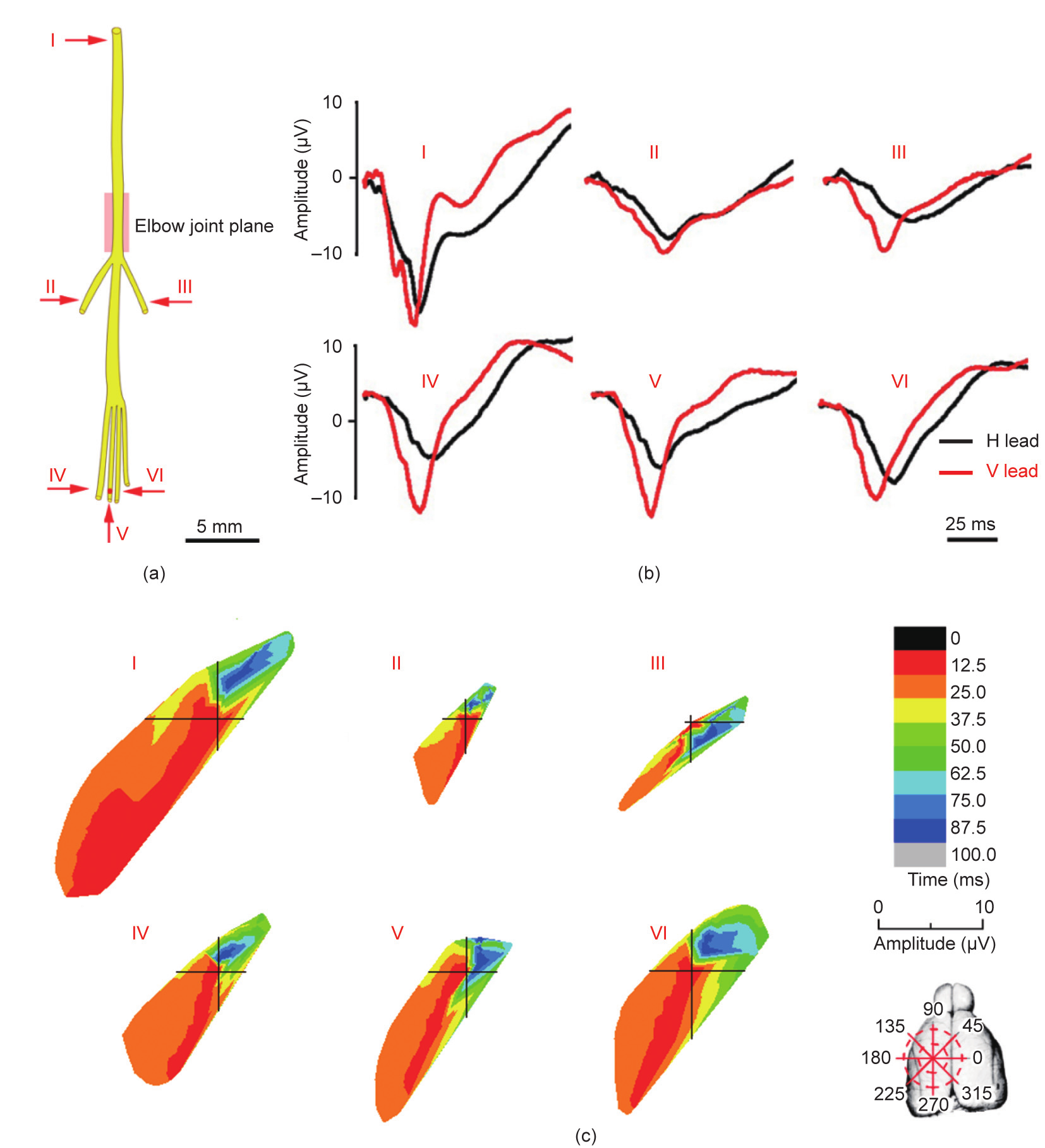
Fig. 3. ECPs induced by the median nerve and its subdivided branches. (a) Sketch map of the median nerve and arrows indicate the stimulating points. (b) The ECP waveform of the median nerve and its subdivided branches. (c) The temporal–spatial characteristics of the ECP induced by the median nerve and its subdivided branches. I: Median nerve; II: muscular branch of the median nerve; III: anterior interosseous nerve; IV–VI: common palmar digital nerves (radial, median, and ulnar side, respectively).
《Table 1》
Table 1 Parameters of the ECPs induced by the median nerve and its subdivided branches (mean ± SD, n = 6).
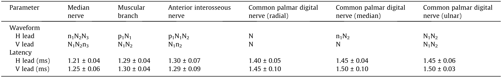
The main ECP wave of the median nerve trunk in the H lead consisted of four consecutive negative waves (n1N2N3N4). The main ECP in the V lead showed a waveform of the N1N2n3 type (Fig. 3 and Table 2).
《Table 2》
Table 2 Parameters of the main ECP waveform of the median nerve trunk in the H and V leads (mean ± SD, n = 6).

The ECPs induced by the median nerve branches (i.e., the muscular branch, anterior interosseous nerve, radial side common palmar digital nerve, median side common palmar digital nerve, and ulnar side common palmar digital nerve) had their own characteristics and could be recognized through specific waveforms (Figs. 3(a) and (b) and Table 1).
In the polar coordinate system, the exciting temporal–spatial sequences of the cortex corresponding to the stimulations of different nerve branches were acquired. For the median nerve trunk, the exciting projection region started from the second quadrant in the first 12.5 ms (ranging from nearly 225° to 240°), which was equivalent to the primary motor cortex (M1) edge. During the next 12.5 ms, the activation area moved to the region ranging from approximately 210° to 225°. Finally, after clockwise spreading, the projection region ended in the first quadrant (87.5–100.0 ms range from nearly 45° to 60°), which corresponded to the secondary motor cortex (M2) edge (Fig. 3(c)). The exciting processes of the cortex induced by different median nerve branches exhibited specific temporal–spatial characteristics (Figs. 3(b) and (c)).
《3.3. Temporal–spatial characteristics of ECPs induced by the ulnar nerve and its subdivided branches》
3.3. Temporal–spatial characteristics of ECPs induced by the ulnar nerve and its subdivided branches
The latencies in the H and V leads of the ulnar nerve trunk were respectively (1.30 ± 0.06) and (1.25 ± 0.04) ms (Fig. 4 and Table 3). Unlike the median nerve, the main ECP wave of the ulnar nerve trunk in the H lead presented as the n1N2 type, consisting of a plateau between the two consecutive negative waves (n1 and N2). The main ECP wave in the V lead was the n1p1N2 type (Fig. 4 and Table 4).
《Fig. 4》

Fig. 4. ECPs induced by the ulnar nerve and its subdivided branches. (a) Sketch map of the ulnar nerve and arrows indicate the stimulating points. (b) The ECP waveform of the ulnar nerve and its subdivided branches. (c) The temporal–spatial characteristics of the ECP induced by the ulnar nerve and its subdivided branches. I: Ulnar nerve; II and III: dorsal digital nerves (radial and ulnar side, respectively); IV and V: cutaneous branches (radial and ulnar side, respectively).
When branches of the ulnar nerve (i.e., two dorsal digital nerves and two cutaneous branches) were stimulated, the ECP waveforms in the H lead all presented as N type, while those in the V lead exhibited a complex type (Fig. 4 and Table 3).
《Table 3》
Table 3 Parameters of the ECPs induced by the ulnar nerve and its subdivided branches (mean ± SD, n = 6)

《Table 4》
Table 4 Parameters of main ECP waveform of the ulnar nerve trunk in the H and V leads (mean ± SD, n = 6).

The ECP vector of the ulnar nerve trunk started from the area between the second and the first quadrants in the first 12.5 ms (around 170° to 210°), which was the edge of the M1. In the next 12.5 ms, the activating area moved to both sides of the initial exciting region from approximately 225° to 250° and from 150° to 170°. Finally, after bidirectional spread, the exciting region ended in the first quadrant (30° to 65°), which corresponded to the M2 edge (Fig. 4(c)). The exciting processes of the cortex areas corresponding to each branched ulnar nerve exhibited different temporal–spatial characteristics (Fig. 4(c)).
《3.4. Temporal–spatial characteristics of ECPs induced by the radial nerve and its subdivided branches》
3.4. Temporal–spatial characteristics of ECPs induced by the radial nerve and its subdivided branches
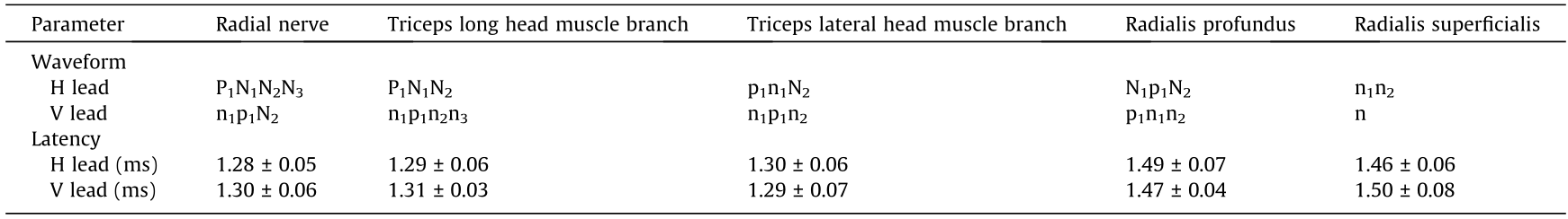
The latencies of the ECP in the H and V leads of the radial nerve trunk were respectively (1.28 ± 0.05) and (1.30 ± 0.06) ms (Table 5). The main ECP wave of the radial nerve trunk in the H lead began with a remarkable positive wave (P1), followed by three consecutive negative waves (P1N1N2N3). The main ECP waveform in the V lead was of the n1p1N2 type. (Figs. 5(a) and (b) and Table 6). Most of the ECPs induced by the branches of the radial nerve in the H lead (i.e., the triceps long head muscle branch, triceps lateral head muscle branch, radialis profundus, and radialis superficialis) had a distinct initial positive wave (Table 5).
《Table 5》
Table 5 Parameters of the ECPs induced by the radial nerve and its subdivided branches (mean ± SD, n = 6).
《Fig. 5》
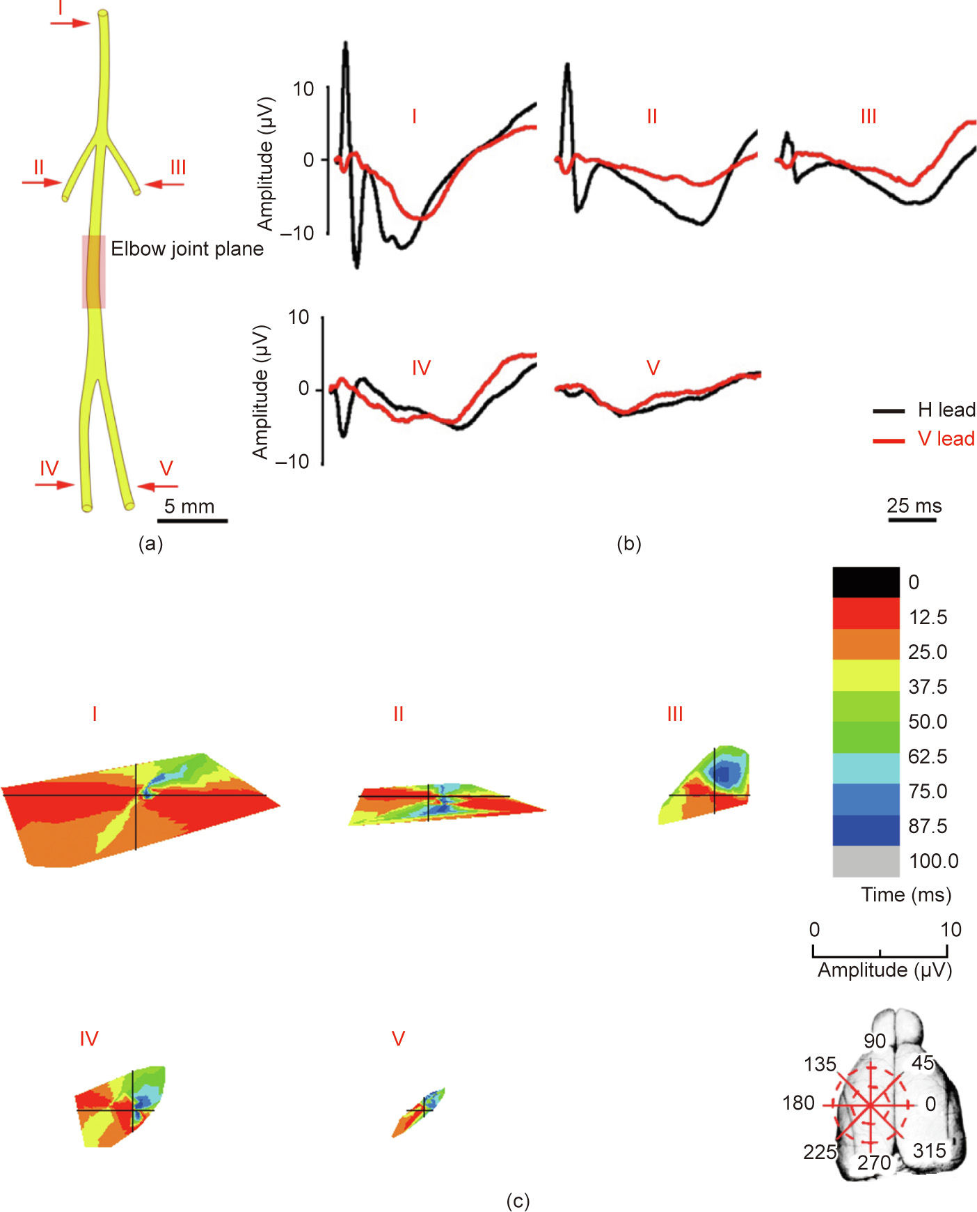
Fig. 5. ECPs induced by the radial nerve and its subdivided branches. (a) Sketch map of the radial nerve and arrows indicate the stimulating points. (b) The ECP waveform of the radial nerve and its subdivided branches. (c) Temporal–spatial sequences analysis of the radial nerve and its subdivided branches in the orthogonal lead system. I: Radial nerve; II: branch to the long head of the triceps muscle of the radial nerve; III: branch to the lateral head of the triceps muscle of the radial nerve; IV: radialis profundus; V: radialis superficialis.
The exciting spatial distribution in the cortex induced by the radial nerve trunk was shaped like a rectangle. It started from the top and bottom areas of the original site in the first 12.5 ms (from 170° to 210° and from 310° to 360°), which was close to the edge of the M1. During the next 12.5 ms, the ECP signal spread to both sides next to the initial exciting region (from approximately 210° to 300° and small area near 160° and 10°). Finally, after bidirectional spread, the excitatory signal ended in the first quadrant (from nearly 30° to 60°, at the M2) (Fig. 5(c)). The exciting processes of the cortex areas corresponding to each radial nerve branch exhibited specific temporal–spatial characteristics (Fig. 5(c)).
《Table 6》
Table 6 Parameters of main ECP waveform of the radial nerve trunk in the H and V leads (mean ± SD, n = 6).

《3.5. ECP temporal–spatial change after median nerve damage》
3.5. ECP temporal–spatial change after median nerve damage
Upon re-examination four months after the median nerve transection, significant changes occurred in the temporal–spatial characteristics and waveforms of the ECPs when stimulating the ulnar and radial nerve trunks using the same method as before. The main ECP waveform of the ulnar nerve trunk in the H lead changed into the n1N2N3 type, compared with the n1N2 type in normal rats. In the V lead, it changed into the N1N2 type, compared with the initial n1p1N2 type (Table 7). For the radial nerve, the ECP waveforms in the H and V leads became P1N1N2 and n1p1n2, respectively, in comparison with P1N1N2N3 and n1p1N2, respectively, before the operation (Table 8).
《Table 7》
Table 7 Waveforms and latency time of the ulnar nerve trunk after median nerve transection (mean ± SD, n = 6).

《Table 8》
Table 8 Waveform and latency time of the radial nerve trunk after median nerve transection (mean ± SD, n = 6).

Although the shape of the excitatory region evoked by the ulnar nerve four months after the operation remained triangular, the distribution area showed a tendency to extend to the median nerve evoked regions. The distribution area started from the third quadrant in the first 12.5 ms (from 235° to 250°, at the M1). In the following 12.5 ms, the excitatory area moved anti-clockwise to the areas (approximately 225° to 230°). Finally, after clockwise spreading, the excitatory region ended in a small area at the first and second quadrants (330° to 360° and 0° to 30°), which corresponded to the M2 (Fig. 6). For the radial nerve, the excitation progress retained its original pattern. However, the amplitude of the ECP vectors increased significantly after the median nerve injury (Fig. 7).
《Fig. 6》
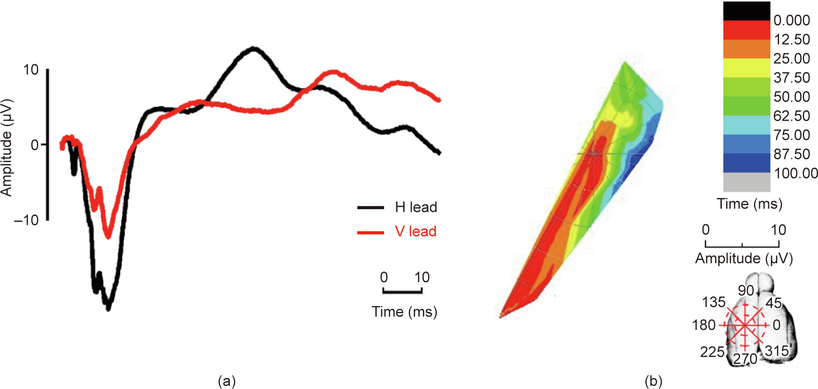
Fig. 6. Temporal–spatial change of the ECP induced by the ulnar nerve four months after median nerve transection. (a) The ECP waveform and (b) temporal–spatial sequences of the ulnar nerve.
《Fig. 7》
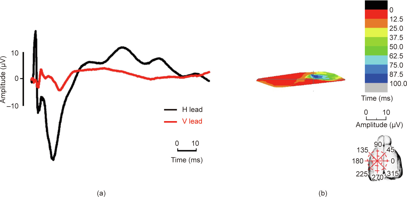
Fig. 7. Temporal–spatial change of the ECP induced by the radial nerve four months after median nerve transection. (a) The ECP waveform and (b) temporal–spatial sequences of the radial nerve.
《4. Discussion》
4. Discussion
In this research, we developed a novel electrophysiological method with an orthogonal lead system and mini-invasive procedures that can acquire the resultant ECPs and temporal–spatial sequences in response to stimulations of peripheral nerves. A ten-year brain research plan was recently proposed by the United States’ government to overcome limitations in brain research caused by fragmental knowledge of the nervous system [28–31]. In that plan, an important research field is the development of new techniques in order to understand complex brain functions in as integral a way as possible [30,32,33]. Traditional electrophysiological methods can only measure the nerve conduction velocity and the evoked potentials to determine the continuity between the peripheral nerves and the brain [34]. It is difficult to monitor and analyze the complicated functional relationship between the peripheral and central nervous systems. The method developed herein provides a way to continuously capture the overall ECP signals corresponding to stimulations of the peripheral nerves. These complicated signals are then decomposed into multiple orthogonal spaces, so that the resultant brain electrical signals can be extensively analyzed into time and space components. In this way, the functional states of multiple brain cortical regions in different phases could be viewed by the researchers. Our work significantly overcomes the inevitable defects in traditional methods such as poor stability and reproducibility, serious individual variation, and limited representation; thus, the present study represents a great step forward in reflecting the overall functional processes and characteristics of the brain.
A typical ECP atlas corresponding to the different peripheral nerves and subdivided branches was first obtained using the method presented herein. According to the ECP atlas results, a peripheral nerve or branch can easily be distinguished by its typical waveform. As described in the results, stimulation of the radial nerve evoked three consecutive negative waves following a large amplitude pre-phase positive wave in the H lead (P1N1N2N3), while the ECP of the ulnar nerve consisted of a small negative wave following a deep negative wave with a small slope in the H lead (n1N2). Similar results were observed in the other small nerve branches. Moreover, the parameters of the ECP, such as latency time, amplitude, and wave composition, were highly relative to the states of neural function such as nerve conductive velocity, exciting degrees, and distribution of activated cellular populations (Fig. 8). Therefore, it was possible to analyze the characteristics of the waveform, and then determine the status and interaction between the peripheral nerve and the brain cortex. This method is similar to the use of an electrocardiogram to interpret the working status of the heart. Thus, the highly recognizable ECP atlas can be used to analyze advanced brain functions.
《Fig. 8》
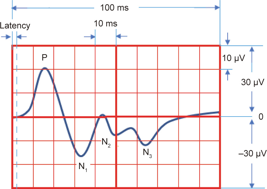
Fig. 8. A theoretical model diagram of the ECP evoked by stimulation of the radial nerve. The ECP induced by a specific nerve stimulation exhibits distinguished and repeatable parameter characteristics, including latency time, amplitude, and wave composition.
The method described above allowed us to visualize the temporal–spatial properties and the precise progress of the brain in response to specific peripheral nerve stimulation and reconstruction. According to our results, the ECP vectors of the median nerve are mainly located in the M1 and lateral M2. Furthermore, the detailed excitation progress from the lateral M1 spreading clockwise to the M1/M2 border was captured and visualized step by step in time and space. The excitation progress in the cortex of the radial and ulnar nerves and their branches was also represented herein. When the brain performs an action, different sets of neurons depolarize, repolarize, or have their membrane potential changed in a coordinate manner. The location and time phase of the ECP vectors projected in the orthogonal plane indicated the space distributions of different functional cell populations in the brain cortex and the time sequences of the relevant neuron groups involved in the reaction. Therefore, this method allowed the researchers to precisely observe and analyze the detailed exciting space–time sequences of the brain visually.
Major discoveries in scientific analysis—such as the ECP atlas and visualizations of exciting sequences in the cortex in response to peripheral stimulations reported here—are primarily useful for obtaining an understanding of the working programs and reaction patterns of the brain and for generating new hypotheses. The results obtained by the method presented here have generated a number of clues to be investigated in future studies. The observed exciting sequences of the projected cortex areas specific to different nerves indicate complex neuro signal transferring progresses and responding mechanisms in the brain. The data described here provide a basis for power analyses for subsequent studies, and the ECP atlas provided here can serve as a baseline reference for other researches. Variations in the ECP waves and temporal–spatial sequences would then suggest typical pathological and physiological processes in nerve function change and brain remodeling. As shown in Figs. 6 and 7, the tendency of ECPs extending to the median nerve projection areas was observed in the cortex after median nerve transection. More detailed progress could be examined in greater depth.
In conclusion, this study provides a novel method for exploring the overall functional connection and remodeling mechanisms between the peripheral and central nervous systems. The precise and reproducible temporal–spatial response of the brain to peripheral stimulation has been obtained for the first time. This method is simple and stable with excellent reproducibility and trivial individual variations. It provides a wealth of information and a basis for systematic analyses of the functional connections between the peripheral and central nervous systems. This resource can serve as a testbed to study the dynamic interactions of the brain and peripheral nerve reconstructions over time. However, there is a lack of exact analyses of the physiological meaning of each wave component. The parameters obtained in this study were all obtained under anesthesia; although the stimulation of each peripheral nerve showed a unique repetitive brain feedback waveform, these should be different from those in a normal physiological state. Future studies will address these problems in more detail.
《Acknowledgments》
Acknowledgments
This work was supported by the National Natural Science Foundation of China (82072162 and 81971177) and the Beijing Municipal Natural Science Foundation (7192215).
《Compliance with ethics guidelines》
Compliance with ethics guidelines
Xiaofeng Yin, Jiuxu Deng, Bo Chen, Bo Jin, Xinyi Gu, Zhidan Qi, Kunpeng Leng, and Baoguo Jiang declare that they have no conflict of interest or financial conflicts to disclose.


 京公网安备 11010502051620号


