《1. Introduction》

1. Introduction

Vibration control (also known as vibration suppression or isolation) refers to a family of techniques for the protection of primary structures or systems against excessive vibrations induced by dynamic loads. Vibration control is widely utilized in aerospace, mechanical, and civil structures for noise control [1], vehicle suspension-related applications [2,3], satellite vibration suppression [4], and protection of large-scale civil infrastructures against extreme earthquakes and typhoons [5]. Existing vibration control techniques are generally categorized as passive, semi-active, or active techniques [6], each of which possesses unique advantages and disadvantages. Passive control devices, which do not require any feedback systems and power input, suppress undesired vibrations by modifying the inherent structural properties and/or dissipating structural kinetic energy. In contrast, active control offers the best control performance by exerting optimized active control forces based on feedback signals. However, its high power demand hinders its application in controlling large-scale structures (e.g., civil infrastructure), particularly considering the limited power availability in remote locations. Semi-active control lies between passive and active controls; it can typically achieve a more efficient control performance than its passive counterpart but consumes less input power than its active counterpart. Table 1 summarizes the conventional views on the three types of vibration control techniques.

《Table 1 》

Table 1 Comparison of different types of vibration control techniques.

However, these conventional views are being increasingly challenged by the latest technological developments in the field of structural vibration control. For example, the power demands of passive and semi-active controls have recently been redefined via emerging vibration-based energy harvesting technology. The introduction of dual-functional dampers with simultaneous vibration damping and energy harvesting functions presents the exciting advancement of passive dampers from energy dissipating to energy regenerating mode (i.e., from zero to negative power consumption), wherein electromagnetic (EM) dampers enable the conversion of kinetic energy to electric energy, and the latter is further stored in capacitors or rechargeable batteries for later use [7,8]. Given the adoption of EM dampers in existing vibration control devices (such as EM mass dampers or driver systems [9,10], EM shunt dampers [11], and EM inerter dampers [12,13]), such an energy harvesting paradigm can be conveniently introduced in a variety of vibration control applications. For example, energy regenerative tuned mass dampers (TMDs) have been developed for high-rise buildings by combining classical TMDs and energy harvesting passive dampers [7,14]. Zhang et al. [15] reviewed the recent developments and investigations on energy regenerative shock absorbers. The energy regenerative braking system for electric vehicles represents another important application field of such energy harvesting passive damping devices [16–19].

Researchers have also started to explore self-powered semiactive vibration control technologies. For example, Cho et al. [20] proposed a combination of a magnetorheological (MR) damper and an EM induction device, wherein the latter served as a power source for the former. This self-powered semi-active control system was later tested in a laboratory experiment on a full-scale cable [21]. Chen and Liao [22] further upgraded the mentioned prototype by integrating the EM and MR components and verified the system experimentally.

Developing self-powered active vibration control presents a more revolutionary and challenging task. The existing attempts were mainly focused on two strategies. The first involves using two separate units to perform energy-harvesting and active control functions, similar to that of the aforementioned semi-active solution. Scruggs and Iwan [23] proposed an energy-regenerative actuation network that extracts vibration energy from one location and applies it to another location. Suda et al. [24] explored a selfpowered active vehicle suspension with an energy-harvesting motor installed in the primary suspension and another active EM actuator installed in the secondary suspension. The second strategy involves operating control devices alternately in passive (energyharvesting) and active (energy-consuming) modes. Nakano and Suda [25] subsequently applied the same system design (Ref. [24]) to a suspension for a truck cabin. Tang and Zuo [26] utilized an active TMD to develop clipped linear–quadratic–Gaussian (LQG) control algorithms. However, in these two strategies, active control still needs to rely on an additional power source; otherwise, the active control force cannot be fully produced. Therefore, neither of these two strategies can be regarded as a truly self-powered active vibration control strategy.

The feasibility of a truly self-powered active vibration control system remains to be proven. Accordingly, we should first revisit the power flow in an active vibration control system. Fig. 1 shows a representative force–velocity relationship produced using an actively controlled actuator in a vibration isolation system. If the curve is in the first and third quadrants, the transient power of the active actuator is positive (i.e., power-harvesting), whereas if the curve is in the second and fourth quadrants, the transient power is negative (i.e., power-consuming). Therefore, if the enclosed area in the first and third quadrants is greater than that in the other two quadrants, the net output power will be positive (Fig. 1). Can we extend this conclusion to a generic vibration control case? Notably, active vibration control refers to a special subset of structural control technology with the unique goal of minimizing the vibration energy of a host structure. To prevent any control instability problem, an overall energy injection into the host structure (i.e., negative net output energy) should be avoided, although a negative transient power flow is allowable. Thus, theoretically, the active control can be self-powered if the transient output power can be efficiently stored and utilized subsequently in the vibration cycles.

《Fig. 1》

Fig. 1. Typical control force–velocity relationship in an active vibration isolation system. Q: quadrant.

The realization of such a concept, which will certainly involve more challenges and will be more complex than the above ideal situation, has never been explored. This paper presents the first attempt to develop a novel self-powered active vibration control system. The topology, working mechanism, and a power analysis of the system are first introduced and discussed herein. The proposed system was then implemented on an active vibration isolation table using the classical skyhook control algorithm. Subsequently, the active control performance and self-powered feasibility were successfully validated through numerical and experimental investigations.

《2. Self-powered active actuator design》

2. Self-powered active actuator design

《2.1. System topology》

2.1. System topology

Fig. 2 shows a single-degree-of-freedom (SDOF) vibration isolation system with the proposed self-powered actively controlled actuator under seismic excitation. The self-powered active control system comprises four modules: an EM actuator, an H-bridgebased power electronics circuit with a rechargeable battery, a microcontroller unit (MCU), and a sensory system.

《Fig. 2》

Fig. 2. Schematic of the proposed self-powered active control system. m_h: isolated mass of the host structure; k_h: stiffness of the host structure; c_h: damping coefficient of the host structure; Acc: acceleration; Vel: velocity; F_ctrl: control force; A and B: two nodes of the EM device; M₁–M₄: four metal-oxide-semiconductor field-effect transistors (MOSFETs); Arduino: the open-source MCU platform (https://www.arduino.cc/); R₀: the inner resistor; L₀: the inner inductor; Sig 1 and Sig 2: pulse-width modulation (PWM) signals.

The EM actuator can produce a control force compatible with large-scale structures [27,28]. In the circuit model, the EM actuator is represented by a back electromotive force (EMF, V_m) and by the inner resistor (R₀) and inductor (L₀) of the coil. The relative motion of the EM actuator generates EMF, while the current (i) passing through the EM actuator generates the control force (F_ctrl).

where K_em is the motor constant, which is solely dependent on the properties of the EM actuator; and are the absolute velocities of the structure and ground, respectively; and represents the relative velocity experienced by the EM actuator. The negative sign of F_ctrl indicates that a positive current will result in a downward force on the isolated mass (m_h).

The MCU determines the target control force based on the received sensing signals and translates it into pulse-width modulation (PWM) signals to manipulate the H-bridge circuit. In this study, an open-source MCU platform (Arduino Uno) was employed to fulfill the integrated functions of data sensing and acquisition, data processing, control algorithm execution, and data output. The analog sensing signals (including the absolute and relative velocities in this study) were collected and digitalized through an onboard analog to digital (A/D) converter. Then, the control algorithm code was uploaded to Arduino through a C language-based embedded integrated development environment (IDE), which determined the duty cycle of the PWM signals.

The H-bridge circuit allows bidirectional power flow, thereby serving as a typical switch-mode rectifier [29]. Although traditionally used in motor driver circuits, the H-bridge circuit has recently attracted interest in the energy-harvesting field [30]. Liu et al. [31] employed an H-bridge circuit controlled using PWM waves to enhance the energy-harvesting efficiency of piezoelectric materials. A similar H-bridge interface was used to tune EM energy harvesters to improve the energy harvesting efficiency [32,33]. Hsieh et al. [29] adopted an H-bridge topology in an energyregenerative suspension system by emulating various resistances and realizing semi-active skyhook control.

In this study, the H-bridge circuit served as an actuator driver and an energy-harvesting circuit. As shown in Fig. 2, the Hbridge power circuit is the interface between the EM actuator and the rechargeable battery, controlling the charge and discharge of the battery. The H-bridge circuit comprises four metal–oxide– semiconductor field-effect transistors (MOSFETs). Two diagonal MOSFET sets, namely M₁–M₄ and M₂–M₃, were controlled via PWM signals Sig 1 and Sig 2, respectively, and each diagonal set was switched on and off simultaneously at a high alternating frequency (starting from thousands of hertz). Four N-type MOSFETs (i.e., N-MOS) were adopted in this study and were ‘‘on” only when the PWM signals on their gate nodes were at high levels (i.e., over threshold voltage (V_GS)). Considering the voltage fluctuation at nodes A and B in Fig. 2, high-side MOSFETs (i.e., M₁ and M₃) require an extra bootstrap circuit or a gate driver for control.

Meanwhile, the rechargeable battery served as both a powerstorage and power-supply element. Apart from rechargeable batteries, supercapacitors are frequently used in energy-harvesting applications. However, since a rechargeable battery can maintain a more stable voltage (V_batt) than a supercapacitor, nickel–metal hydride (Ni-MH) batteries were adopted in the proof-of-concept tests in this study.

《2.2. System principle》

2.2. System principle

To avoid short-circuit-induced damage to the system, Sig 1 and Sig 2 can not be at high levels simultaneously, and thus the two diagonal sets are alternated between ‘‘on” and ‘‘off.” Consequently, the duty cycles (D₁ and D₂) of Sig 1 and Sig 2 should satisfy the approximate relationship D₁ + D₂ = 1. If the switching period of the PWM signals is T_PWM = 1/, where is the PWM frequency, then M₁ and M₄ are on (Sig 1 is high), and M₂ and M₃ are off (Sig 2 is low) during t₁ = T_PWM·D₁. Consequently, node A connects to the positive pin of the power source, and node B connects to the ground. When the control signal flips in a PWM cycle, Sig 1 is low and Sig 2 is high for the remaining duration of t₂ = T_PWM·(1 – D₁).

If the current (i) in the actuator and the inductor is assumed to be positive when flowing from right to left, then each switching cycle has the following relationships according to Kirchhoff’s voltage law:

where V_m is the instantaneous EMF, V_batt is the voltage of the rechargeable battery, and R_total is the total circuit resistance, including the motor inner resistance (R₀) and the resistances of the battery, connecting wires, and other electrical elements (e.g., MOSFETs). In each PWM cycle with an extremely short duration, V_m and V_batt can be regarded as nearly constant, current i is in a steady state, and the total change in the current should be nearly zero. Consequently, the current flowing through the EM actuator can be estimated by solving Eqs. (2) and (3), as follows:

According to Eq. (1), the current generates a control force when passing through the EM motor:

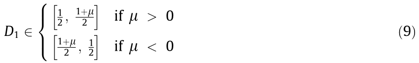
Given that D₁ [0, 1], the achievable ranges of the current and control forces are as follows:

Eq. (6) reveals that the achievable current range can be increased using a larger power source voltage (V_batt).

A laboratory experiment was conducted to verify the relationship in Eq. (4). In this experiment, the EM actuator was represented by the combination of an inductor (L₀ = 0.1 H), a resistor (R_total = 16 Ω), and a battery (V_m = 2.5 V) that emulates a constant EMF. The voltage of the rechargeable battery (V_batt) is 12 V. Four N-MOSs (part No.: IRF840A) were used in the H-bridge, and the drain–source on-resistance of each was only R_MOS = 0.85 Ω, which is considered in the total resistance (R_total) of the entire circuit. The experimental setup was nearly the same as that used in the SDOF test described in Section 3.2, except for the replacement of the EM actuator with a battery (i.e., a constant EMF). More detailed descriptions and images of the setup are provided in Section 3.2. Fig. 3 displays the relationship between the actuator current and duty cycle D₁, whose theoretical result is based on Eq. (4). The simulation result was generated using the MATLAB Simulink toolbox. The consistency observed in Fig. 3 confirms the accuracy of Eq. (4) and the Simulink model.

《Fig. 3》

Fig. 3. Relationship between the current of the actuator and the duty cycle (D₁) of the control signal. μ = V_m/V_batt.

Fig. 4 shows a schematic of the relationship between the control force (–F_ctrl) and the relative velocity experienced by the EM actuator. As predicted using Eq. (5), the upper and lower bounds, corresponding to D₁ = 0 and 1, respectively, define the achievable range of the control force. Any desirable active control force within this range can be generated by regulating D₁ accordingly. The achievable range of the control force can be increased by adopting a larger power source voltage (V_batt), a larger motor constant (K_em), and a reduced circuit resistance (R_total).

《Fig. 4》

Fig. 4. Partition of power-consuming and power-harvesting zones in the plane of active control force versus relative velocity of the actuator.

《2.3. Power analysis》

2.3. Power analysis

In this section, the power flow between the EM actuator and the rechargeable battery is discussed. Within a short PWM cycle, the current (i) flowing in the EM actuator, which is defined in Eq. (4), remains nearly constant; the current in the battery has the same amplitude but flows in both directions owing to the switching of the H-bridge circuit. Consequently, if the current (i) in the EM actuator is positive (from right to left), the battery is charged and discharged during t₁ and t₂, respectively. Power harvesting or consumption depends on the relative durations of t₁ and t₂. Thus, the average output power (P) within one PWM cycle, which is termed the instantaneous output power hereinafter, can be calculated as follows:

Substituting Eq. (4) into Eq. (7) yields

The instantaneous output power (P) is positive when the actuator harvests power and negative when it injects power back to the structure. Eq. (7) reveals that the power exchange between the EM motor and rechargeable battery is governed by the duty cycle of the H-bridge circuit. The duty cycle for the positive instantaneous output power can be obtained as follows:

where μ = V_m/V_batt. The corresponding condition for the current (i) flowing in the EM actuator can be obtained using Eq. (8).

The green shaded area in Fig. 3 shows the derived powerharvesting range when μ > 0 (i.e., V_m > 0).

Substituting Eqs. (1) and (4) into Eq. (10) leads to the following power-harvesting condition in the force–velocity relation:

The green shaded area in Fig. 4 denotes the power-harvesting zone in the actuator force–velocity plane, while the yellow area represents the power-consuming zone. The boundary is defined by a straight line with a slope of , which corresponds to the duty cycle of D₁ = 0.5 and zero output power. Compared with Fig. 1, the power-harvesting zone is reduced from the first and third quadrants to two sectors owing to the total circuit resistance (R_total). A minimal R_total value that can enlarge the powerharvesting (i.e., green) zone in Fig. 4 is desirable.

However, the force–velocity relationship does not always fall in the green zone. To realize a self-powered active vibration control system, the average output power should remain positive over a given period.

The dashed loop in Fig. 4 indicates a representative control force–velocity relation in a vibration cycle. As long as the force– velocity loop covers more of the green area than of the yellow area, the active actuator can operate in an overall energy-harvesting mode. The rechargeable battery stores the harvested power temporarily in the green zone and reuses this power in the yellow zone to generate active control forces.

Notably, the foregoing derivation is based on the assumption that the structural vibration frequency is considerably lower than the switch frequency of the H-bridge; the former typically ranges from less than one hertz to hundreds of hertz, whereas the latter typically exceeds thousands of hertz. Otherwise, the control force would not be successfully achieved through the proposed setup.

《3. Active vibration isolation with self-powered actuator》

3. Active vibration isolation with self-powered actuator

The SDOF vibration isolation system with the proposed selfpowered active actuator (Fig. 2) was investigated numerically and experimentally to verify the vibration control and power performance. The skyhook control algorithm was employed to determine the active control force.

《3.1. Numerical modeling and control algorithm》

3.1. Numerical modeling and control algorithm

The equation of motion for the SDOF structure shown in Fig. 2 can be expressed as

where m_h, c_h, and k_h represent the mass, damping, and stiffness coefficients of the isolated structure, respectively; x, , and are the absolute displacement, velocity, and acceleration of the structure, respectively; and are the ground input displacement and velocity, respectively; and F_ctrl is the active control force. The above equation can be rewritten in a state-space form as

The classical skyhook control, which represents an ideal vibration isolation with a hypothetical viscous damper connecting the sprung mass to an immobile ceiling [34], was adopted to determine the active control force:

where c_sky denotes the damping coefficient of the hypothetical damper. The active control performance improved with increasing c_sky. Different c_sky values were considered in this study to achieve different levels of control performance.

Consequently, the transmissibility function (H) of the isolated structure with the skyhook controller could be derived as follows:

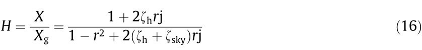
where X and X_g are the Fourier transform of x and x_g, respectively; r = ω/ω_n is the ratio of the ground motion frequency (ω) to the natural frequency for the host structure ;  and  are the damping ratios contributed by the structure damping and skyhook control, respectively; and j =  is the imaginary unit. 

Combining Eqs. (5) and (15) provides the duty cycle required to produce the target control force.

The generated duty cycle (D₁) is then passed to the H-bridge circuit to deliver the control force required by the skyhook control. Although only skyhook control was adopted in this study, the presented methodology can be easily applied to any other active control algorithm.

Fig. 5 shows a block diagram of the entire active control system, including the state-space model of the host structure, the ideal skyhook control, the feedforward control algorithm to determine the duty cycle, the H-bridge circuit, and the EM actuator. In addition to the EM force, the parasitic force of the EM actuator is considered in this diagram. The total control force of the EM actuator exerted on the host structure formed a closed loop.

《Fig. 5》

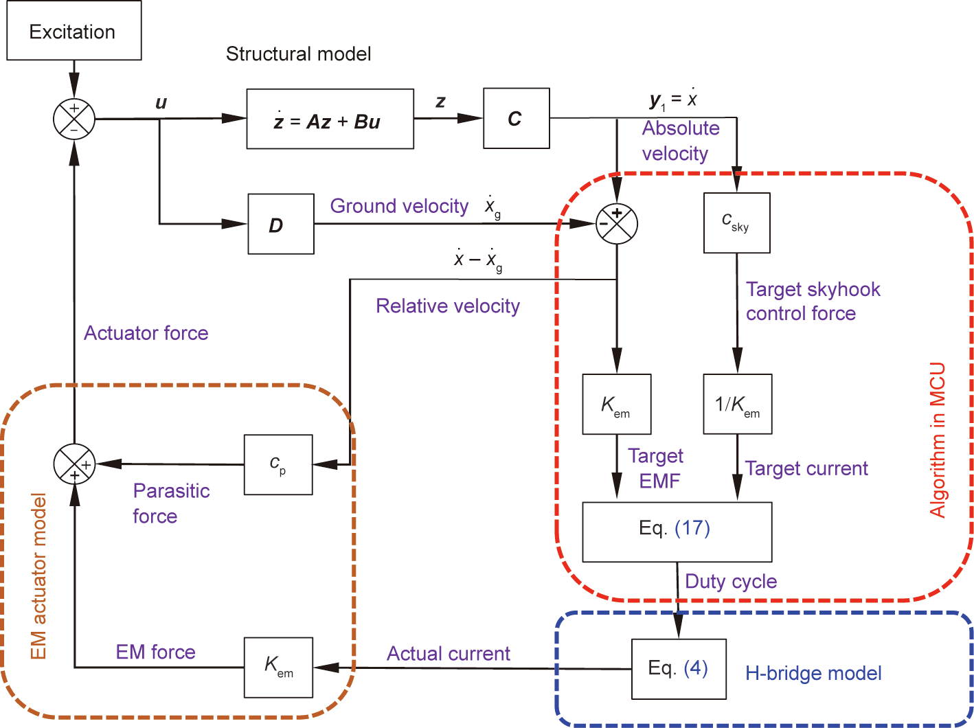
Fig. 5. Block diagram showing the self-powered active vibration isolation system with skyhook control algorithm. A, B, C, D, z, u, and y represent state matrix, input matrix, output matrix, feedforward matrix, state vector, input vector, and output vector, respectively; c_p is parasitic damping coefficient.

When the SDOF structure is subjected to harmonic ground excitation, 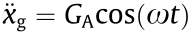where G_A stands for amplitude of the ground motion, the instantaneous output power can be calculated by substituting Eqs. (1), (4), (15), and (16) into Eq. (8):

where H is the transfer function seen in Eq. (16). Consequently, the average output power (energy transferred to or consumed from the battery) within one vibration cycle can be calculated as

where T = 2π/ω is the period of the harmonic excitation.

Fig. 6 shows the entire self-powered active vibration isolation system modeled in MATLAB Simulink. The major parameters of the mechanical and electrical components were modeled in accordance with those used in the experiment. The simulated PWM frequency was 2 kHz, and the computation timestep of the Simulink model was set to 10^–6 s to ensure sufficient points within each duty cycle. Numerical simulations were performed to verify the theoretical results and guide the laboratory experimental design.

《Fig. 6》

Fig. 6. Simulink model of the self-powered active vibration isolation system. Fcn: MATLAB function module; tgt: target; DC: duty cycle; PID: proportional–integral– derivative; s: saturation.

《3.2. Experimental setup》

3.2. Experimental setup

Fig. 7 presents an overview of the experimental setup for the active vibration isolation plate (i.e., the SDOF system). The three main components (i.e., control module, H-bridge module, and SDOF system) are highlighted with gray rectangles.

《Fig. 7》

Fig. 7. Overview of experimental setup. The meanings of the 16 pins of HIP4082 chip can be found in the corresponding data sheet https://www.renesas.com/ www/doc/datasheet/hip4082.pdf (AHB and BHB: the high-side bootstrap supply of A and B nodes; AHS and BHS: the high-side source connection of A and B nodes; AHI, BHI, ALI, BLI, AHO, BHO, ALO, and BLO: the high-side and low-side, input and output of A and B nodes, respectively; V_SS and V_DD: negative and positive supply to control logic and lower gate drivers, respectively; DEL: turn-on delay; DIS: disable input; GND: ground; VCC: voltage common collector; R₁: a 10 kΩ resistor).

The vibration isolation plate consisted of a mass plate (#4 in Fig. 8) suspended by four vertical springs (#2), representing an SDOF structure oscillating in the vertical direction. The input signal from the signal generator was first amplified using a power amplifier and then used to drive a 355 mm × 355 mm shake table to excite the SDOF structure with the designed ground motions. An EM motor was installed between the mass plate and the shake table, functioning as a control actuator (EM motor B in Fig. 8).

The absolute acceleration of the mass plate was measured using two accelerometers installed on the plate. The absolute velocity was subsequently obtained through real-time integration of the acceleration signals using an anti-aliasing signal convertor. The relative velocity between the isolated mass plate and shake table was measured using another EM motor, denoted as the sensing motor (i.e., EM motor A in Fig. 8). Given that the top plate was rigidly connected to the shake table, the two EM motors were installed in parallel with each other and experienced the same relative velocity. In addition, the current flowing in the EM control motor was recorded by measuring the voltage difference across a small-value sensing resistor (R_s = 1 Ω).

《Fig. 8》

Fig. 8. (a) Photo and (b) schematic drawing of the experimental setup of the vibration isolation table. 1: top plate; 2: spring; 3: load cell; 4: mass plate; 5: EM motor A (sensing); 6: fixture; 7: accelerometers; 8: EM motor B (actuation); 9: base plate.

The adopted MCU was an Arduino Uno board (Italy) with an ATmega328 (USA) microcontroller (clock speed of 16 MHz), 14 digital input/output (I/O) pins, and four analog input pins. Its typical power consumption was approximately 250 mW. The power consumption can be significantly reduced by using other low-power MCUs, such as an Arduino Pro mini (Italy) or even a tailor-made MCU with all unnecessary parts and functions removed. The aforementioned absolute velocity of the mass plate, the open-circuit voltage of the EM sensing motor, and the current in the circuit were sensed by the MCU at a sampling frequency of 200 Hz. The MCU processed the sensing data and executed the control algorithm shown in the ‘‘MCU” block in Figs. 5 and 6. The control algorithm was coded in an open-source C language-based IDE provided by Arduino AG. The MCU outputs the PWM signal with a determined duty cycle (D₁) at the switching frequency of 2 kHz, corresponding to the PWM cycle of 500 μs.

The two nodes of the EM control motor, denoted as Nodes A and B in Figs. 2, 7, and 8, were connected to the H-bridge circuit and hence to the rechargeable battery set. Fig. 9 shows the printed circuit board (PCB) layout and a photograph of the manufactured PCB (35 mm × 60 mm) hosting the H-bridge circuit. The H-bridge comprised four N-MOSs, which were controlled through a full-bridge driver as shown in Fig. 7. This full-bridge driver was adopted mainly to trigger high-side MOSFETs that experienced fluctuating voltages at their source pins. The full-bridge driver received PWM signals from the MCU. The value of R₁ in Fig. 7 controls the deadtime between two inverted PWM signals and thus prevents short circuits. According to the user manual, R₁ = 10 kΩ, which was selected in this study, corresponds to a deadtime of 0.5 μs. The battery set comprised three Ni-MH batteries connected in series, providing a nominal voltage of 12 V. An additional inductor was incorporated into the circuit to increase the motor inductance (L₀) and smoothen the current curve.

《Fig. 9》

Fig. 9. H-bridge module. (a) PCB layout and (b) image of the PCB prototype. PolyU CEE: Department of Civil and Environmental Engineering, The Hong Kong Polytechnic University.

In addition to the sensing signals utilized in the feedback control, more sensors were installed to evaluate the vibration control and power performance. An additional accelerometer was installed to measure the input acceleration of the shake table. Two laser displacement transducers were used to measure the absolute displacement of the mass plate and the shake table. A load cell was used to measure the control force of the EM actuator. The sensing data were collected using a data acquisition system at a sampling frequency of 10 kHz. Meanwhile, the charge and discharge currents of the battery were measured using a separate data acquisition system at a sampling frequency of up to 100 kHz, which is 50 times the PWM switching frequency; this enabled determination of the duty cycle of the PWM signals.

The major parameters of the experimental setup are summarized in Table 2, while the model numbers of the major equipment and items are presented in Table 3. The vibration isolation table was tested under harmonic ground accelerations with a constant acceleration amplitude of 0.18g and varying excitation frequencies of 3–15 Hz. Two damping coefficients, c_sky = 20 and 40 N·s·m^–1 , were implemented individually in the skyhook controller. The vibration control and power performance were evaluated in these test scenarios.

《Table 2 》

Table 2 Major parameters of the tested active vibration isolation system.

^a The total mass includes the masses of the isolated plate, the moving parts of the EM motors, the accelerometers, and other auxiliary elements installed on the plate.

^b The parasitic damping coefficient stands for the inherent damping of the EM motors with open circuit. The parasitic damping also affects system dynamic behaviors.

^c 1 rad = 180°/π.

《Table 3 》

Table 3 Model numbers of the equipment and items used in the experiment.

《3.3. Influence of time delay》

3.3. Influence of time delay

Fig. 10 displays a comparison between the experimental and target EM control forces. The former was calculated using Eq. (1) and the measured motor current, while the latter is the product of the measured absolute velocity of the mass plate and the coefficient c_sky = 40 N·s·m^–1 . Although the experimental control force matches the amplitude of the target control force very closely, an approximate time delay of = 0.01 s can be observed in this comparison. This delay is likely due to data processing, which involves sampling, A/D conversion, transmission, synchronization, and control algorithm execution. A typical method to mitigate the influence of the time delay is to use a compensator (such as a proportional–integral–derivative (PID) controller). However, no compensator was implemented in the control algorithm, as the influence of the time delay was insignificant in this study.

《Fig. 10》

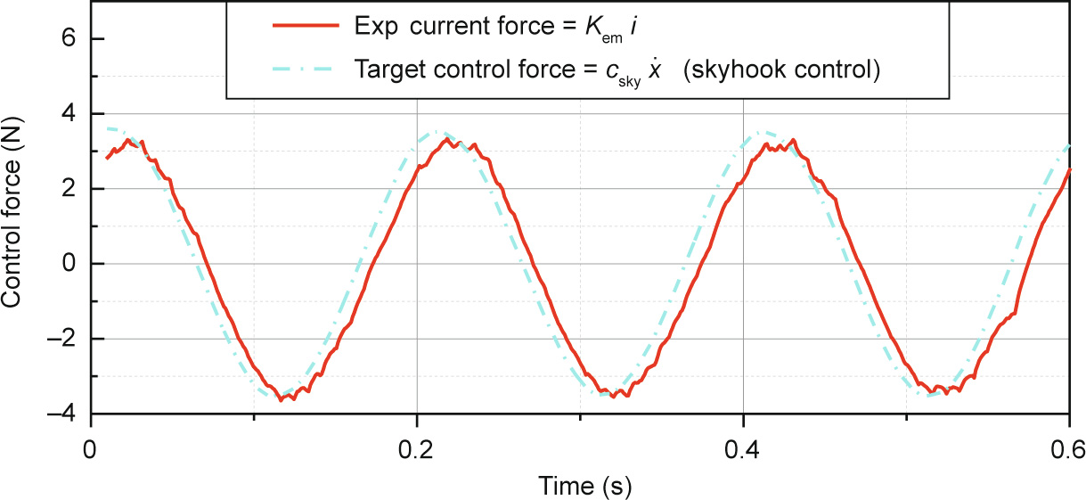
Fig. 10. Comparison of the measured and target control forces in time domain (c_sky = 40 N·s·m^–1 , excitation frequency = 5 Hz, sampling frequency = 10 kHz). Exp: experimental.

Considering the time lag in the active control force, the theoretical transmissibility function in Eq. (16) can be rewritten as

The impact of the time delay is frequency-dependent and thus becomes more significant under high-frequency excitation. The time delay was also considered in the Simulink model by adding a delay module before the control force was applied to the host structure, as shown in Fig. 6 (bottom left module). The theoretical transmissibility formula and the numerical model, considering the time delay, represent more realistic descriptions of the dynamics of the active vibration isolation system, from which the results can be better compared with the data from the experiment.

《3.4. Power analysis》

3.4. Power analysis

Fig. 11 shows the time histories of the currents through the EM actuator and the rechargeable battery, together with the calculated power flow in an experimental case with the skyhook coefficient of c_sky = 40 N·s·m^–1 and excitation frequency of 5 Hz.

The green dashed line in Fig. 11(a) represents the EMF divided by the circuit resistance R_total. Thus, the corresponding shaded area represents the energy-harvesting region according to Eq. (11). The EM actuator alternately operates in the power-harvesting and power-consuming modes when the actuator current falls inside and outside the shaded area, respectively. The red vertical dotted lines mark the intersection points of the actuator current (i.e., the orange dashed line) and energy-harvesting region (i.e., green). These vertical lines divide the entire time history into ‘‘powerharvesting” and ‘‘power-consuming” regions, as shown in Fig. 11(a). The blue dashed line shows the battery power calculated as the product of the battery current and voltage; the instantaneous positive and negative powers represent the powerharvesting and power-consuming processes, respectively. Provided that the battery current switches direction (charge and discharge) at a high frequency, the presented power in Fig. 11(a) is the average power over every 0.002 s (around four PWM periods). The points where the calculated instantaneous power equals zero coincide with the vertical red line partitions in the figure. In general, the actuator current in the power-harvesting region is within the green shaded area, and the instantaneous power of the battery is positive (energy-harvesting); conversely, the actuator current in the power-consuming region is outside the shaded area, and the instantaneous transient power of the battery is negative (energyconsuming).

Fig. 11(b) specifically displays the battery current in the time domain corresponding to that in Fig. 11(a). The current in the battery (i.e., the gray solid line) switches direction at the frequency (i.e., 2 kHz) of the PWM control waves; the positive and negative currents within each PWM cycle, which represent the charge and discharge processes of the battery, respectively, have nearly equal magnitudes, while the current in the EM actuator (i.e., the orange dotted line) varies slowly at the vibration frequency (i.e., 5 Hz). The EM actuator current approximately profiles the battery current on one side because the actuator current alternatively connects to the battery in two opposite directions in a PWM cycle.

《Fig. 11》

Fig. 11. Energy exchange between motor and rechargeable battery in time domain (c_sky = 40 N·s·m^–1 , = 5 Hz): (a) actuator current and battery power flow; (b) actuator current and battery current with allocated windows indicating energy consumption and energy harvesting locations; and (c) enlarged windows showing details for energy consumption (①) and energy harvesting (②).

Two representative time windows, denoted as ① and ② in Figs. 11(b) and (c), were selected from the power-consuming and power-harvesting regions. The variation in the measured battery current within one PWM cycle in the selected windows is shown in detail in the enlarged view in Fig. 11(c). The positive and negative currents correspond to the charge and discharge states of the battery, respectively. Both the positive and negative parts were flat and had nearly equal amplitudes. In window ①, the negative current lasted longer than the positive current (D₁ = 42%), reflecting an energy-consuming effect. In window ②, the positive current lasted longer (D₁ = 54%) than the negative current, leading to an energyharvesting effect. The enlarged windows also show that the smoothed actuator current is approximately equal to the amplitude of the battery current, although the latter exhibits more significant fluctuations.

Fig. 12 displays plots of the experimental and simulation relations of the control forces versus the relative velocities of the EM actuator obtained in two representative experimental cases, with Fig. 12(a) c_sky = 40 N·s·m^–1 , = 3 Hz and Fig. 12(b) c_sky = 40 N·s·m^–1 , = 7 Hz, which correspond to the energy-consumption and energyharvesting scenarios, respectively. The total damper force directly measured using the load cell included the EM and parasitic damping forces. The former represents a control force, while the latter is uncontrollable. The experimental EM control force was calculated based on the measured actuator current using Eq. (1). In general, the simulated EM force is consistent with the experimental EM force, demonstrating the accuracy of the numerical model presented in Section 3.3 that considers the time delay effect.

The instantaneous power-harvesting and power-consuming zones depicted in Fig. 4 are also highlighted in Fig. 12. The elliptical control force–velocity loops in Figs. 12(a) and (b) pass through both the power-harvesting and power-consuming zones. Most of the elliptical force–velocity loop in Fig. 12(a) is located outside the green shaded area. According to Eq. (11), the average output powers in this case were estimated to be –80 and –59 mW for experimental and numerical results, respectively, demonstrating that the active EM actuator consumed energy overall. In contrast, the loop shown in Fig. 12(b) mainly lies in the green shaded area. The average output powers obtained from the experimental and numerical results were 8 and 3.6 mW, respectively. The positive output power suggests that the actively controlled actuator harvested energy overall.

《Fig. 12》

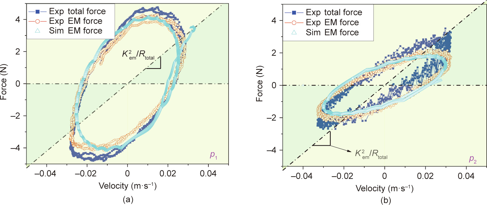
Fig. 12. Experimental results showing ranges of energy harvesting and energy dissipation. (a) Energy harvesting (c_sky = 40 N·s·m^–1 , = 3 Hz); (b) energy consumption (c_sky = 40 N·s·m^–1 , = 7 Hz). Sim: simulation; p₁ and p₂ match the two points marked in Figs. 13 and 14.

Fig. 13 plots the theoretical, simulation, and experimental results of the average output power obtained in all cases. The theoretical curves were obtained using Eq. (19). The satisfactory agreement among the three results validates the efficacy of the theoretical and numerical models. In general, the vibration isolation performance improved with an increase in the skyhook damping coefficient c_sky, but the average output power decreased. The two points p₁ and p₂ in Fig. 13 correspond to 3 and 7 Hz, respectively, matching the force–velocity diagrams in Figs. 12(a) and (b).

《Fig. 13》

Fig. 13. Average output power of the active vibration isolation system with skyhook control. Theo: theoretical.

Within the resonant frequency range of 6–10 Hz (the corresponding frequency ratio r [0.8, 1.4]), where excellent vibration control performance is required, active vibration isolation based on the skyhook algorithm could be successfully achieved in the energy-harvesting mode. However, in the low-frequency range (r < 0.7), the active isolation system operated in an energyconsuming mode. When the frequency ratio r > 2.07, although the theoretical result predicts a positive output power, the numerical and experimental results present an output power that is slightly less than zero owing to the extra power loss in the Hbridge circuit.

Thus, the self-powering feature was not realized in all of the experimental cases. This situation can be improved by minimizing the total resistance (R_total) of the circuit, which will enlarge the power-harvesting zone in Fig. 13. In addition, the superior active control performance is highly desirable in the resonant region, while outside the resonant region, the vibration isolation performance becomes less sensitive to c_sky. Hence, a lower c_sky value can be adopted to achieve a tradeoff between energy and vibration control performance outside the resonant region.

The foregoing power-balance discussion only considered the instantaneous power of the EM actuator. The additional power consumption of the sensors and MCU were not considered. However, only a small-scale structure was tested in this proof-ofconcept study. In large-scale structural control applications, the power consumption of the sensing and MCU units is negligible compared with the instantaneous vibration power from structures.

《3.5. Control performance》

3.5. Control performance

Fig. 14 shows the transmissibility curves of the actively isolated structure obtained in the theoretical and experimental studies under various conditions. The solid green line indicates the uncontrolled baseline case with only parasitic damping. The black dotted lines represent the transmissibility curves of the passive control group, with passive viscous dampers (c_sky = 20 and 40 N·s·m^–1 ) installed between the structure and the ground. The red dashed lines show the theoretical curves of the ideal skyhook control as defined in Eq. (16), while the blue dash-dot lines represent the theoretical curves of the skyhook control, considering the time delay effect, as defined in Eq. (20). A comparison of these two groups illustrates the slightly negative impact of the time delay, particularly in the high-frequency range. Additionally, the two investigated points ( p₁ and p₂) are circled in pink.

《Fig. 14》

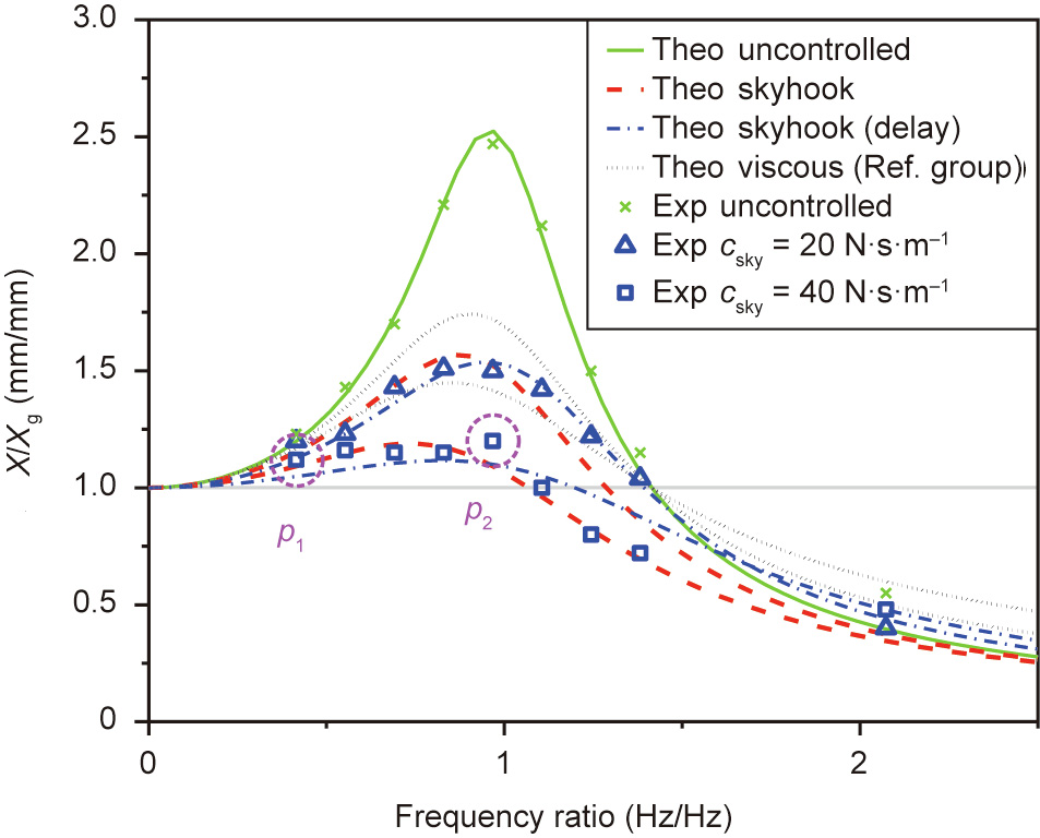
Fig. 14. Transmissibility curves under skyhook control.

The experimental control performance corresponding to the two damping coefficients, c_sky = 20 and 40 N·s·m^–1 , satisfactorily agrees with the corresponding theoretical performance. This validates the successful active skyhook control performance. In general, active skyhook control can yield superior isolation performance over its passive counterparts. Considering c_sky = 40 N·s·m^–1, the resonant peak became indistinct in the corresponding transmissibility curves.

《4. Conclusions》

4. Conclusions

This paper proposed an unprecedented self-powered active vibration control strategy to overcome the power supply bottleneck associated with conventional active vibration control techniques. The system design, working mechanism, power flow, control algorithm, and performance of the strategy were presented and discussed based on analytical, numerical, and experimental studies. The feasibility and effectiveness of the proposed system were examined by applying it to an active vibration isolation system. The results obtained in this study indicate that manipulating the duty cycles of PWM control signals according to the derived relation can not only enable accurate production of the target active control force but also allow the EM actuator to operate alternately in different power modes (power-harvesting or powerconsumption). Consequently, a truly self-powered active vibration isolation system was successfully achieved for the first time, and the classical skyhook vibration isolation could be realized without any external power supply to the EM actuator.

Although the skyhook control algorithm was adopted in this study to illustrate the feasibility of the self-powered concept, the proposed strategy and setup present a generic solution that can be readily extended to other active vibration control applications with versatile active control algorithms, by simply modifying the sensing signals and updating the control algorithm code executed by the MCU. Therefore, the proposed self-powered strategy can have a profound impact on existing active vibration control techniques in a wide range of applications.

《Acknowledgments》

Acknowledgments

This work was supported by the Research Grants Council of Hong Kong through General Research Fund (GRF) projects (15214620 and PolyU 152246/18E), Research Impact Fund (PolyU R5020-18), and the NSFC/RGC Joint Research Scheme (N_PolyU533/17 and 51761165022).

《Compliance with ethics guidelines》

Compliance with ethics guidelines

Jin-Yang Li and Songye Zhu declare that they have no conflicts of interest or financial conflicts to disclose.