
《1. Introduction 》
1. Introduction
With the development of global economies and the increasing demand for modernization in construction, tunnels have become one of the optimal choices for traffic infrastructure construction in complex geological terrains. The geological conditions of the surrounding rock in a tunnel construction environment are complex, and various geological disasters, such as a collapse or water inrush, are often caused by unfavorable geological bodies, such as karsts and fracture zones. Because tunnel construction occurs in the geological body, there can be a substantial number of casualties and property losses during construction if the unfavorable geological bodies (belt) around the tunnel are not accurately predicted [1]. Therefore, it is critical to detect hidden geological hazards ahead of the tunnel face in advance to reduce the hidden dangers and ensure the safety of the construction site.
Advanced tunnel detection is a type of geophysical technology used to detect hidden geological hazards ahead of the tunnel face using observation systems. Current geophysical methods used for advanced tunnel detection primarily include seismic, electromagnetic, electrical, and geological radar methods [2–5], among which the tunnel seismic detection method has become common for its long detection range and accurate for the prediction. This technique is based on the difference in the seismic wave velocity between abnormal geological bodies and the surrounding rock. During construction, as seismic waves are transmitted to the surrounding rock of the tunnel and the collected seismic data is processed, the distribution of abnormal geological bodies ahead of the tunnel face and the mechanical parameters of the rock are obtained for an early warning and guidance during tunnel construction. In the late 1970s, engineers in Germany and England explored the geological structure ahead of the tunnel working face by using the airy seismic phase of the channel wave. In the early 1990s, the Swiss Surveying Technology Co., Ltd. developed a set of advanced tunnel seismic prediction (TSP) systems. In the late 1990s, a US engineering company developed the true reflection tomography (TRT) technology, Zeng [6] and Inazaki et al. [7] proposed the vertical seismic profile method for tunnels, then developed into application by Zhao et al. [8] and Alimoradi et al. [9] at the beginning of 21st century. Based on the increase in tunnel construction, the currently available seismic advanced geological prediction methods include the TSP, horizontal seismic profiling (HSP), TRT, tunnel seismic tomography (TST), tunnel seismic while drilling (TSWD), tunnel geology prediction (TGP), and the negative apparent velocity method of seismic waves [10–15]. However, the observation system is limited to the tunnel environment, and the amount of data collected cannot meet the requirements of a high calculation accuracy for the tunnel geological body wave velocity. The imaging results obtained using the tunnel seismic detection method cannot accurately detect abnormal geological bodies. This method is only suitable for simple geological conditions [16]. More accurate detection methods suitable for advanced tunnel geological prediction are necessary.
The development of full-waveform inversion (FWI), which is an inversion technique that uses full wave field information to invert medium parameters in the seismic exploration field, has provided several opportunities. In the 1980s, researchers proposed a timedomain FWI based on the least-squares method and introduced this concept to the seismic exploration field [17–19]. Compared to the traditional inversion method that uses a single reflected wave or the first arrival wave data to obtain the attributed parameter imaging, FWI fully utilizes the full wave field information to achieve a higher resolution [20]. Therefore, this high-precision and high-resolution inversion method has been significantly praised for seismic wave field inversion and reconstruction and has gained increasing attention in the research and application of seismic velocity modeling [21,22]. Owing to the nonlinearity and cycle-skipping of FWI, the objective function has multiple local minima, which makes the inversion significantly dependent on the initial model [23–25]. To reduce the dependence of the inversion results on the initial model, early researchers proposed a multi-scale FWI method in the time domain that filters the seismic data to isolate frequencies [26]. In the 1990s, Pratt and Worthington [27] extended the theory of frequency-domain FWI. The inversion results of the low-frequency components in the frequency-domain FWI can be used as the initial model of the high-frequency components, which can directly achieve the effect of multi-scale inversion and reduce the dependence on the initial model [27–31]. Owing to this advantage, the frequency-domain FWI is widely used in seismic exploration.
For advanced tunnel detection applications, Musayev et al. [32,33] first applied the full waveform inversion method in the frequency domain to tunnel and discussed whether the full waveform can successfully image the velocity field in a tunnel. Nguyen and Nestorovic´ [34,35] proposed a global optimization procedure for the FWI of two-dimensional (2D) tunnel seismic waves; they also used the elastic FWI enhanced with the parametric representation for locating the disturbance zones ahead of a tunnel face. Bharadwaj et al. [36] developed a seismic prediction system to enable imaging ahead of a tunnel-boring machine. Lamert et al. [37] proposed two flexible elastic time-domain FWI methods to predict the disturbance area ahead of a tunnel face. As a local case study, Zhang et al. [38] used the FWI method with ground penetrating radar (GPR) to distinguish unfavorable geological bodies within 20 m ahead of a tunnel face. Li [39] used the acoustic FWI method to predict the velocity interface of large geological bodies ahead of a tunnel face. Feng et al. [40] improved the reconstruction of tunnel lining defects using GPR profiles with FWI.
Considering that the environment owns a limited tunnel seismic detection space and observation coverage, to improve the accuracy of tunnel seismic detection, we tested the frequencydomain acoustic FWI method for tunnel seismic detection. Using the abnormal low-speed body as example, we constructed a tunnel low-speed body model and its observation system based on the tunnel space and reconstructed the tunnel velocity model with frequency-domain acoustic FWI. By comparing different frequency group selection strategies of frequency-domain FWI, we analyzed the results of the frequency group selection and determined suitable options for the tunnel seismic method. Herein, we discuss the influence of the side length of the tunnel observation system on the inversion. Finally, we used a complex tunnel geological model to verify the effectiveness of the method and the parameter selection strategy.
《2. Frequency-domain acoustic FWI 》
2. Frequency-domain acoustic FWI
《2.1. Theory of 2D frequency-domain acoustic FWI》
2.1. Theory of 2D frequency-domain acoustic FWI
In an isotropic medium, the 2D acoustic wave equation in the frequency domain is expressed as follows [41]:

where k(x, z) is the bulk modulus, ρ(x, z) is the density, d(x, z, ω) is the pressure field, (x, z) represents the 2D coordinates, ω is the frequency, and s(x, z, ω) is the source function.
Because the pressure field d(x, z, ω) is linear with respect to the source s(x, z, ω), the discretized 2D acoustic wave equation can be simplified into the following large sparse linear equation:

where A represents the impedance matrix of the frequency and medium properties. Considering that d(x, z, ω) and s(x, z, ω) are stored as vectors of dimension Nx ×Nz, A(ω) is a finite difference operator matrix of (Nx,Nz) ×(Nx,Nz), which can be solved using the lower–upper (LU) decomposition method. The wave equation (Eq. (1)) is discretized by the mixed-grid finite–difference (FD) method; in addition, the perfectly matched layer (PML) absorbing boundary condition is used to simulate the virtual boundary in the model and the free surface at the inner tunnel surface [42,43].
We use the L2 norm as our frequency-domain acoustic FWI’s objective function; it is given by the squared difference between the observed and calculated data, as follows:

where Nω is the number of frequencies in the group, Ns represents the number of sources, Nr represents the number of receivers, dobs(s, r, ω) is the observed wave field, and dcal(s, r, ω) is the calculated wave field using the parameters of model m, H is conjugate transpose. E(m) is a function related to the model parameter m, and its gradient is calculated as follows:

where J T is the transpose of the Jacobian matrix, which is derived from the partial derivatives of the wave field on the model parameters.  is the complex conjugation of the wave field residuals, and Re is the real part of the complex number. The gradient of E(m) is calculated to obtain the perturbation of the model parameters in iterations to minimize the misfit between the observed and calculated wave fields [44]. The inversion error threshold and iteration number are set as the termination conditions for updating the model to ensure convergence at a practical cost. The model medium parameters satisfying the conditions are obtained when the inversion is terminated.
《2.2. Strategy for FWI frequency group selection in tunnel space 》
2.2. Strategy for FWI frequency group selection in tunnel space
2.2.1. Strategy for frequency group selection
Frequency-domain FWI allows us to obtain large-scale information by first inverting low-frequency data corresponding to long wavelengths, then the information retrieved from middle- and high-frequency short wavelengths can depict detailed features. In the process of FWI, the low-frequency inversion results are used as the initial model for the subsequent middle- and highfrequency inversions, which can directly reach multi-scale inversion. Because the probability of non-convergence caused by the local extremum of the low-frequency data inversion is small, a relatively good initial model can be estimated, which can improve the convergence stability of the inversion process and accelerate the inversion convergence [45].
In this manner, the selection of frequency groups for the FWI in the frequency domain is worth studying. Sirgue and Pratt [46] conducted a frequency selection method based on the continuity of vertical wavenumber coverage, in which the maximum wavenumber corresponding to the frequency value of the current stage should be equal to the minimum wavenumber corresponding to the frequency value of the next frequency stage, as follows:

where  represents the frequency value of the current stage,
  is the frequency value of the next frequency stage, and the vertical wavenumber kz is the vertical component of the wavenumber vector k. The range of kz depends on the incident angle of the seismic wave and its relationship with the calculation results in the following equation:

where α is the cosine of the maximum incident angle, hmax is the maximum half offset of the current observation system, and z is the depth of the reflection layer.
An extensive offset, high-density geophone distribution observation system, and horizontal reflecting strata are apparently required. However, the observation system of the tunnel space is limited, and the geological conditions of tunnels are often complex. This strategy can only obtain limited depth information ahead of the tunnel face. In addition, to satisfy the antialiasing condition, the sampling rate of the vertical wavenumber  should satisfy ≤ 1/zmax [47,48]. Then, the relationship between the vertical wave number and background velocity in the calculation can be used to obtain the following formula:

where c0 is the velocity of the background,  represents the frequency value between two frequency stage intervals, and zmax is the maximum imaging depth.
This strategy for frequency sampling has been proven to have wider application possibilities, despite the relatively slow convergence rate of inversion due to the decrease in sampling points in the low-frequency region.
2.2.2. Strategy for frequency group selection of tunnel FWI
Tunnel seismic detection systems often have a limited offset of observation and its records own a large frequency distribution range with a high dominant frequency. Therefore, the frequency selection strategies in Section 2.2.1 are no longer applicable in the tunnel space. To improve the inversion resolution of tunnel FWI, we propose a method that combines the advantages of both as follows:

In addition, we suggest using the background velocity  for the elastic FWI.
Eq. (8) is a combined formula as shown in Fig. 1, in the lowfrequency range, it is used to obtain a more detailed lowfrequency group to ensure the large-scale inversion effect of the model. Eq. (7) is used as the judgment condition in Eq. (8), when the frequency group obtained cannot satisfy the antialiasing criterion, a constant frequency interval is chosen to ensure it.
《Fig. 1》
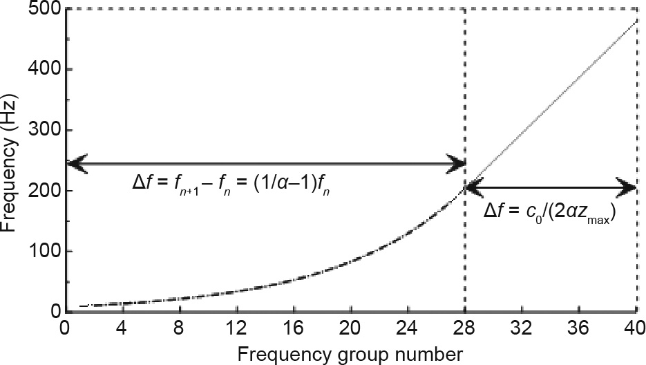
Fig. 1. Frequency group curve. In the beginning frequency range, the frequency interval  increases linearly with the frequency group number, when increasing to a threshold the frequency increases with equal to satisfy the antialiasing condition.
《3. Discussion of parameters and calculation results 》
3. Discussion of parameters and calculation results
《3.1. Observation system and model design》
3.1. Observation system and model design
The tunnel seismic detection method arranges excitation holes in the tunnel face and the sidewalls with depths of 0.5 or 1.0 m. Seismic waves propagate to the wall rock of the tunnel through artificial excitation. When the impedance of these waves changes, part of the seismic waves will be reflected, and the other part continues to spread forward. The reflected seismic waves are recorded by the receivers and provide the seismic records. The processed records can predict geological changes ahead of the tunnel face and provide reliable geological data for tunnel construction [49,50]. Based on actual tunnel parameters, we built the tunnel low-speed anomalies model shown in Fig. 2(a), which is 200 m (X axis) ×30 m (Z axis), with a 100 m tunnel length and a 12 m tunnel face (width), along with three anomalies with a radius of 3 m located 14, 46, and 84 m ahead of the tunnel face. The tunnel space is full of air, the rock wall velocity is 4000 m·s–1 , and the velocity of the anomalies is 3000 m·s–1 . The observation system of the tunnel seismic detection was set as U-shaped, as shown in Fig. 2(b), including the tunnel face and both sidewalls. With a 1 m excitation hole depth, 57 shot points and 112 receivers are arranged from 51 to 101 m in the sidewalls and tunnel face with a 2 m shot interval length and a 1 m receiver interval length. In the forward modeling, the dominant frequency of the Ricker wavelet is 200 Hz; Figs. 2(c)–(e) present the real part of the monofrequency pressure field slices of 50, 200, and 450 Hz. As indicated, when the velocity remains unchanged and the frequency increases, the wavelength of a single frequency slice in the frequency domain becomes shorter, the difference between the wavelength of the low-velocity anomaly body and that of the wall rock increases, and the details regarding the anomalous body position become more apparent.
《Fig. 2》

Fig. 2. Tunnel model with observation system design and real parts of the pressure field in the frequency-domain. (a) Low speed anomalies model with a tunnel, where X is the length of the tunnel model and Z is the width. (b) Observation system of a tunnel seismic detection. (c)–(e) Real part of a mono-frequency slice for 50, 200, and 450 Hz with shot point located in the middle of the tunnel face.
With a sampling interval of 0.5 ms and a recording length of 160 ms, the acoustic wave pressure component records in the time-domain were obtained through the inverse Fourier transform from the frequency-domain. The shot point in Fig. 3(a) is located at coordinates (51, 9), which is the beginning of the observation system on the side of the tunnel. The shot point in Fig. 3(b) is located in the middle of the tunnel face with coordinates (102, 15). These records contain direct waves and diffracted waves caused by the interface of three low velocity anomalous bodies.
《Fig. 3》

Fig. 3. Records of two shot points for the designed model. (a) Records of Fig. 2(a) with a shot point located the side of the tunnel. (b) Records of Fig. 2(a) with the shot point located at the middle of the tunnel face. These records contain direct waves and diffracted waves caused by the interface of three low velocity anomalous bodies.
《3.2. Discussion of different frequency selection strategies》
3.2. Discussion of different frequency selection strategies
Because low-frequency inversion provides long-wavelength information while high-frequency provides detailed wave propagation information, multi-scale FWI using the low-frequency inversion result as the initial model to invert for the higher frequency data helps the high-frequency inversion converge as well as describe the details [51]. Using the observation system shown in Fig. 2(b), a frequency-domain acoustic FWI of the abnormal tunnel body model, shown in Fig. 2(a), was conducted. The forward simulation in the inversion process adopts a Ricker wavelet with a dominant frequency of 200 Hz. A homogeneous velocity model with a velocity of 3000 m·s–1 was selected as the initial model. Based on the frequency spectrum of the Ricker wavelet, three frequencies (50, 200, and 450 Hz) were selected from low to high. We obtained three root mean square error (RMSE) convergence curves and velocity models after the inversion, as shown in Fig. 4.
《Fig. 4》

Fig. 4. Iteration of multi-frequency inversion. (a) Iteration curves for the inversion of three frequency groups; inversion result of frequencies of (b) 50 Hz, (c) 50 and 200 Hz, and (d) 50, 200, and 450 Hz. (a) demonstrates the convergence process of three frequencies in the iteration, and (b)–(d) describe the process of the multi-scale inversion results from low to high frequency, in which the inversion results can be observed from determining the location of the abnormal bodies.
Based on Eqs. (6)–(8), three frequency groups between 10 and 500 Hz were obtained. To compare the results of the inversion frequency selection strategy, the frequency group obtained by Eq. (6) is named S, while Eq. (7) describes the W frequency group, and Eq. (8) describes the C frequency group. The wavelet spectrum and frequency group parameter curves are shown in Figs. 5(a) and (b), respectively.
《Fig. 5》

Fig. 5. Parameters for acoustic FWI. (a) Ricker wavelet spectrum of the source wavelet; (b) parameters of three frequency groups. Based on Fig. 5(a), the frequency range from 10 to 500 Hz were obtained.
The three frequency groups shown in Fig. 5(b) were used for the FWI with the same initial model shown in Fig. 6(a) and same iterations. The three velocity resolution results are shown in Fig. 6. Figs. 6(b)–(d) W, S, and C frequency groups, respectively. Compared to Fig. 4(d), the inversion respresent the velocity inversion result of theults shown in Figs. 6(b)–(d) are significantly improved; however, the resolution results shown in Figs. 6(b)–(d) remain different. First, we discuss the sensitivity of the velocity inversion result to the location of the abnormal bodies and the imaging accuracy of the inversion results to compare the effects of different frequency selection strategies. The inversion result of the W frequency group showed in Fig. 6(b) is accurate considering the location of the first shallow abnormal body. Additionally, its velocity profile curve has a relatively noticeable disturbance in the position range of the middle and deep abnormal bodies and its adjacent position shown in Fig. 6(e), indicating that the inversion converges beyond the range of the abnormal bodies. The inversion result of group S is relatively accurate for the location of the shallow abnormal bodies shown in Fig. 6(c); the velocity variations in Fig. 6(e) are apparent in the location of the first abnormal body; however, are not as apparent in the location of the middle and deep abnormal bodies. The inversion result of the C frequency group is significantly close to reality in the shallow, middle, and deep abnormal body locations shown in Fig. 6(d), and the velocity curve of the middle profile shown in Fig. 6(e) presents a noticeable and accurate velocity disturbance in the position of the abnormal bodies. Overall, the inversion results obtained by the C frequency group have better convergence sensitivity in the position of the abnormal bodies, which demonstrates the contribution of the frequency group selection to the convergence stability of multi-scale FWI.
The velocity profiles shown in Fig. 6(e) and Fig. 7 are comprehensively compared to discuss the accuracy of the inversion results. The inversion accuracy of the abnormal bodies of the three frequency groups is affected by the distance from the tunnel face, as shown by the comparison velocity profiles; the accuracy worsens with the distance, and the velocity inversion accuracies of the middle and far abnormal bodies are worse than those that are close. A comparison of the three frequency groups reveals that the velocity inversion accuracy of the S frequency group is relatively poor, whereas the velocity inversion accuracy of the W and C frequency groups is better. Their difference in the shallow section is minimal between the inversion results and the initial models, and the inversion result of the C frequency group reflects a higher resolution in the middle and deep sections.
《Fig. 6》

Fig. 6. Initial model and inversion results of different frequency groups. (a) Initial model, (b)–(d) inversion results for models of W, S, C group frequencies obtained by Eqs. (7), (6), and (8) frequency selection strategies, respectively; (e) velocity profile curves in the grid axis Z = 15 of the tunnel models. The comparison of inversion results reveals the difference in the accuracy of inversion results of different frequency group methods for abnormal bodies at different depths.
《Fig. 7》

Fig. 7. Velocity curve comparison of the cross-sections of the three abnormal bodies based on inversion results in Figs. 6(b)–(d). (a) Velocity curve of first abnormal body in grid axis X = 114 of the tunnel models; (b) velocity curve of second abnormal body in grid axis X = 147 of the tunnel models; (c) velocity curve of third abnormal body in grid axis X = 186 of the tunnel models.
In summary, we demonstrated that the frequency-domain acoustic multi-scale FWI based on the tunnel seismic detection method can obtain satisfactory velocity inversion results, and the suitable frequency group selection method proposed in this study can obtain superior resolution results ahead of the tunnel face.
《3.3. Discussion of tunnel model observation system》
3.3. Discussion of tunnel model observation system
To obtain more effective information regarding the geological body ahead of the tunnel face, we suggest using a U-shaped observation system for tunnel seismic detection. Referring to the propagation path of seismic waves in the tunnel space and the energy loss in the process of seismic wave propagation, we consider that the extended range of the observation system on both tunnel sides would no longer affect the inversion results after reaching a certain length. To confirm this, we designed five U-shaped tunnel observation system groups with side lengths of 10, 30, 50, 70, and 90 m, while all other parameters remained constant. The specific inversion results after applying these parameters to the frequencydomain acoustic FWI in the tunnel space are shown in Figs. 8 and 9.
A comparison of Figs. 8(b)–(d) with Fig. 9(a) reveals that the longer the observation system, the more accurate the velocity inversion result. From Figs. 8(d)–(f), when the side length of the tunnel observation system changes beyond a certain range, its influence on the inversion results decreases; increasing the side length has a very weak influence on the inversion results. As demonstrated in the comparison of velocity curves across the tunnel cross-section in Fig. 9(b), the difference between the inversion results of the 70 m side length and that of the 90 m side length is significantly small, and the relative error between them is less than 0.4%. According to the comparison results, for the tunnel face width of this model, considering a built-in geophone and source depth, the optimal resolution results can be obtained by selecting a tunnel observation system with a side length of 70 m.
《Fig. 8》
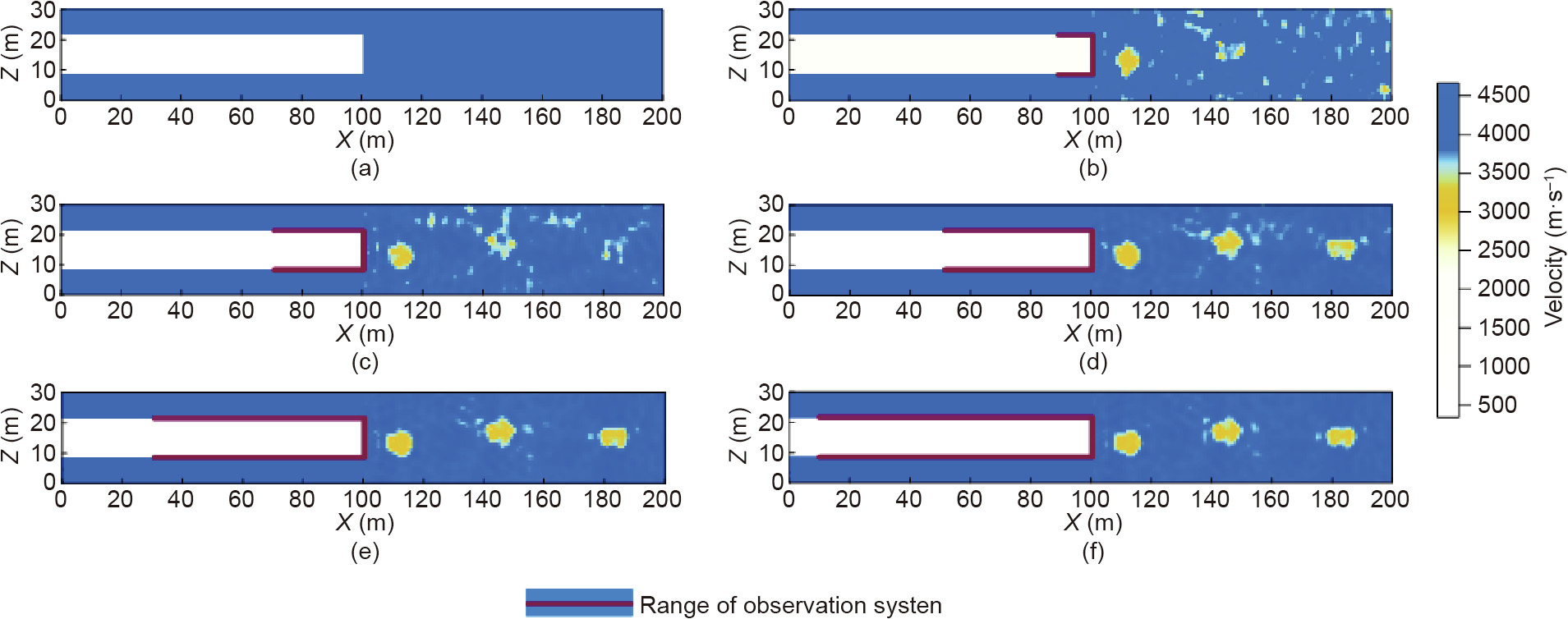
Fig. 8. Initial model and inversion results model of varying tunnel observation system side lengths. (a) Initial model, and (b)–(f) resulting velocity models with 10, 30, 50, 70, and 90 m tunnel observation system side lengths. It can be seen that the velocity results of the same abnormal body obtained by inversion with different observation system and the differences of abnormal bodies with different depths in the inversion results.
《Fig. 9》

Fig. 9. Velocity curve of different tunnel observation system models in axis Z = 15 cross-section based on inversion results in Figs. 8(b)–(f). (a) Velocity results of the side lengths 10, 30, and 50 m, and (b) velocity results of side lengths 50, 70, and 90 m.
Specifically, through multiple comparisons and simulations, we advise that within limits, the longer the arrangement side length of the tunnel observation system, the better the resolution of the inversion result. However, when the side length of the tunnel observation system is more than five times the width of the tunnel face, the influence of increasing the observation system side length on the inversion results is negligible. Overall, this conclusion can potentially aid theoretical studies regarding tunnel FWI and the actual construction of tunnel seismic detection.
《3.4. Complex model calculation and application》
3.4. Complex model calculation and application
To verify the effect of the parameters discussed in this study, a tunnel stratum model including abnormal bodies, low-velocity zones, and complex structures is designed for frequency-domain acoustic FWI based on tunnel seismic detection (Fig. 10(a)).
The true model is designed based on limestone strata with wave velocities of 4500 to 5500 m·s–1 , including low-speed thin-layer abnormal body strata with a velocity of 3000–4000 m·s–1 and other complex geological conditions. The initial model for the forward calculation in the inversion uses the background velocity of the observation model (Fig. 10(b)). The three frequency selection strategies were used as the selection basis for the frequency group parameters to obtain a set of frequencies for the inversion. Using the tunnel observation system with a side length of 70 m as the tunnel observation system, the final velocity inversion results are shown in Figs. 10(c)–(e).
The results of velocity inversion in Figs. 10(c)–(e) demonstrate that the frequency-domain acoustic FWI of the multi-scale strategy can inversely affect the velocity of the shallow sections of the complex tunnel geological conditions, and the closer it is to the tunnel face, the more accurate the results are. For the shallow part, the difference between the inversion results and the true model is minimal in all the three results, whereas the inversion results obtained by the frequency group selection strategy proposed in this study perform better in the middle and deep inversion, which indicates that the resolution in Fig. 10(e) is better than the results provided in Figs. 10(c) and (d).
《Fig. 10》
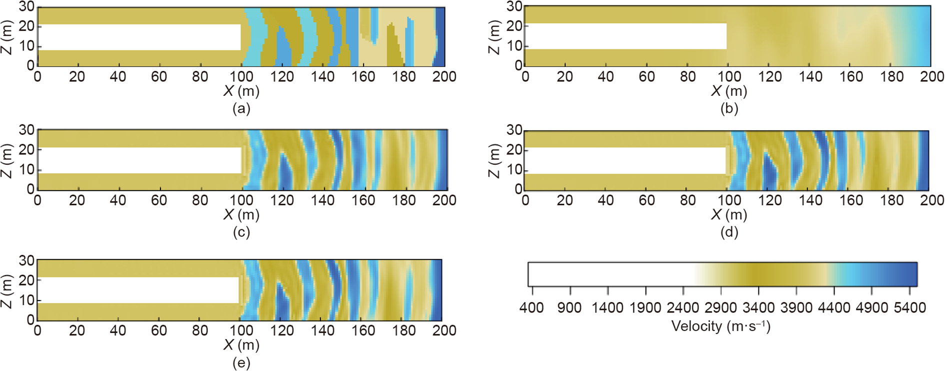
Fig. 10. Comparison of tunnel complex model. (a) True model of tunnel complex model inversion, (b) initial model of tunnel complex model inversion, (c)–(e) inversion result models of W, S, C frequency groups obtained by Eqs. (7), (6), and (8) frequency selection strategies, respectively. For the shallow part, the difference between the inversion results and the true model is minimal in all the three results, whereas the inversion results in (e) performs better in the middle and deep inversion.
Comparing the profile velocities in Figs. 10(e) and (b), Fig. 11(d) indicates that the velocity obtained from the inversion results accurately corresponds to that of the true model, whereas there is a slight misfit at the far side from the tunnel face. The relative error between the inversion result and the real model ranged from 0.3% to 8% in different positions and increased with depth. The error in the near part was the smallest, and that in the furthest position was 6%.
《Fig. 11》

Fig. 11. Velocity comparison of tunnel complex model using C frequency selection strategy. (a)–(c) Velocity model of the initial, true, and result models and (d) velocity profiles of tunnel models from (a)–(c) in the grid axis Z = 15.
The complex geological model inversion results of the frequency-domain acoustic FWI based on tunnel seismic detection prove that the method can successfully invert the stratum information and obtain high-resolution results of complex geological information ahead of the tunnel face under suitable parameters.
For tunnel exploration, all theoretical research and discussions are for practical applications; therefore, we used the TSP observation system with the parameters discussed in this study for a simple field FWI verification. The observation system for the field data acquisition is shown in Fig. 12.
《Fig. 12》
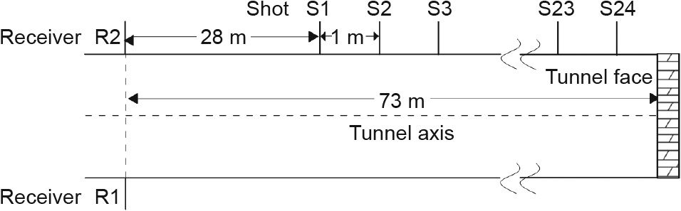
Fig. 12. Tunnel seismic exploration field observation system with two receivers and 24 shot points.
Because the data acquisition is conducted in the time domain, the frequency-domain acoustic FWI requires wave field separation and Fourier transform. Therefore, the X-component field records (Fig. 13(a)) of the TSP were used for filtering and wave field separation to obtain the P-wave component records (Fig. 13(b)) [52], and the direct wave velocity was used as the initial model (Fig. 13 (c)), as shown in Fig. 13(d).
According to the inversion result velocity model in Fig. 13(d), a low-speed zone is located approximately 35–45 m away from the tunnel face with a velocity of 3600 m·s–1 . In the subsequent excavation process, a weak layer with a velocity of 3700 m·s–1 was encountered approximately 30 m ahead of the tunnel face, which proves that the inversion result using the parameters proposed in this study is relatively effective and practical, and will also help to provide a guide for future tunnel construction engineering.
《Fig. 13》
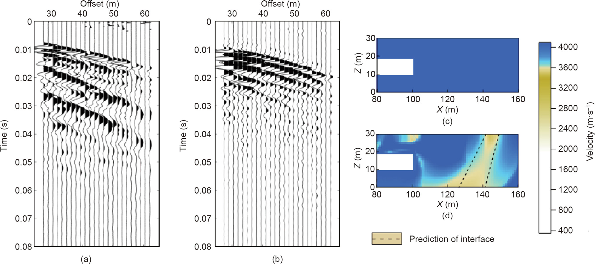
Fig. 13. Tunnel seismic records and the velocity models. (a, b) X-component field records and processed field records of receiver R1, (c) initial model for field data inversion, and (d) inversion result models of the C frequency group selection strategy.
《4. Conclusions》
4. Conclusions
We applied a frequency-domain acoustic FWI to the tunnel seismic detection method and determined the influence of the frequency group selection strategy and tunnel observation system settings. The specific analysis is summarized as follows:
(1) The observation system of the TSP is limited by the tunnel space, and its records have a high dominant frequency with a large frequency distribution range, which makes the common frequency group selection strategies for FWI no longer applicable. Thus, we proposed a strategy for selecting the frequency group under the tunnel detection condition, which uses a frequency group selection strategy combining the low-frequency selection strategy covering the vertical wave number and the high-frequency selection strategy of antialiasing. In comparison, this strategy can obtain a better resolution result ahead of the tunnel face.
(2) Because tunnel construction areas are significantly limited, the U-shaped observation system is widely used in tunnel seismic detection theoretical simulations and practical applications. The Ushaped observation system includes the tunnel face and both sidewalls; however, there is no recommended side length for the FWI of the tunnel seismic detection method. Therefore, in this study, by linearly increasing the side length of the tunnel observation system within limits, if the equipment allows, longer side length arrangements of the tunnel observation system will produce a higher resolution of the inversion result. However, when the side length of the tunnel observation system is more than 5 times the width of the tunnel face, the influence of increasing the observation system side length on the inversion results is negligible.
(3) The results of frequency-domain acoustic FWI of the tunnel seismic detection based on the complex geological model proved that the proposed method can successfully reverse the stratum information ahead of the tunnel face under the parameters discussed and obtain high-resolution results of complex geological information. The practical results of the TSP data further verified the effectiveness and practicality of the parameter selection strategy. This study can provide ideas and references for future theoretical research and practical applications.
《Compliance with ethics guidelines》
Compliance with ethics guidelines
Mingyu Yu, Fei Cheng, Jiangping Liu, Daicheng Peng, and Zhijian Tian declare that they have no conflict of interest or financial conflicts to disclose.
《Acknowledgments》
Acknowledgments
This work was supported by the National Natural Science Foundation of China (41704146) and the Fundamental Research Funds for National Universities, China University of Geosciences (Wuhan) (CUGL180816). We thank the seiscope research group for developing the shared FWI algorithm.


 京公网安备 11010502051620号


