

《1. Introduction》
1. Introduction
Lung cancer causes most cancer deaths in humans, with over 1 million deaths occurring each year worldwide [1]. Approximately 85% of lung cancers are non-small-cell lung cancer (NSCLC), and small-cell lung cancer (SCLC) accounts for 15% of lung cancers [2]. Recently, the chemotherapy-based treatment paradigm for lung cancer patients has shifted with the introduction of driver genes and the advancement of molecular detection technology [3,4], especially in patients with epidermal growth factor receptor (EGFR) gene mutations [5,6] and rearrangements of the anaplastic large-cell lymphoma kinase (ALK) gene [7]. Nevertheless, targeted therapy faces a series of difficulties, including different individual responses and frequent acquired resistance [8,9]. Immune checkpoint inhibitors (ICIs) are recommended for lung cancer patients [10]. However, only approximately 20% of lung cancer patients respond to immunotherapy. It is important to determine the mechanisms of drug resistance in lung cancer patients.
Preclinical animal models are crucial for drug screening. Patient-derived tumor xenografts (PDXs) have emerged as an accurate preclinical system capable of maintaining the molecular, genetic, and histopathologic heterogeneity of parental tumors [11,12]. Moreover, a new generation of super-immunodeficient mice called non-obese diabetic (NOD)/Shi-scid, interleukin-2 receptor (IL-2R)  (NOG) mice, which feature the deletion of the IL-2R common gamma chain and functional deficiency of multiple immune cells (e.g., T cells, B cells, natural killer (NK) cells, macrophages, and dendritic cells), is considered to be an excellent choice for building PDX models for cancer immunotherapy [13]. Compared with nude mice and traditional severe combined immunodeficient (SCID) mice, NOG mice have demonstrated outstanding potential for research on ICIs, adoptive T cell therapy (ACT), and other immunotherapies because tumor-infiltrating T lymphocytes (TILs) can be serially transplanted into them after xenografts develop [14,15].
Nonetheless, the low success rate of PDX establishment (20%– 40%) [16–18] and the notable rate of inconsistent driver gene mutations between established PDXs and the original tumors (10%–20%) [19,20] is a considerable problem that has not been well studied. Since protocols to generate PDX models are timeconsuming, labor-intensive, and costly [21], the inconsistency of driver gene mutations is very problematic for researchers, physicians, and patients. However, multiple factors, including sex, smoking history, pathology, tumor-node-metastasis (TNM) stage, tumor grade, tumor sample quality, and EGFR gene mutations, have been shown to be correlated with the rate of successful tumor engraftment [17,18,22]. Whether these factors contribute to the consistency of driver gene mutations in PDX models, especially those established in NOG mice, has not been validated. This study aimed to use machine learning (ML) algorithms, including multivariable logistic regression (LR), support vector machine (SVM) recursive feature elimination (SVM-RFE), a gradient-boosting decision tree (GBDT), and the synthetic minority oversampling technique (SMOTE) to establish a powerful tool for predicting driver gene mutation inconsistency between NOG/PDX models and patient tumors (Fig. 1).
《Fig. 1》

Fig. 1. Study design and protocol for establishing lung cancer NOG/PDX models and ML. In this study, we initially obtained lung cancer tissues via computed tomography (CT)-guided percutaneous lung biopsy (CT-PLB), lymph node biopsy (LNB), or thoracentesis, and then implanted all tissues into NOG mice. After successfully establishing 53 NOG/PDX models, we took all PDX tissues and then performed hematoxylin and eosin (H&E) staining gene sequencing to confirm whether the genotypes of PDX models matched those of patients’ tumors. We then input 17 clinicopathological features of patients to three ML methods—LR, SVM-RFE, and GBDT. Afterward, we performed five algorithms of these three models, stepwise LR based on the lowest Akaike information criterion (AIC), least absolute shrinkage and selection operator (LASSO)-LR, SVM-RFE, extreme gradient boosting (XGBoost), and gradient boosting and categorical features (CatBoost), to select or rank features among all 53 samples. Next, we generated 100 training groups and 100 testing groups via stratified random sampling. We also exerted the SMOTE to generate ten more positive classes whose genotypes were different from those of the parental tumors and added them into every training group. Finally, we compared the overall performance of each algorithm after training in corresponding training groups.
《2. Materials and methods》
2. Materials and methods
《2.1. Patient samples》
2.1. Patient samples
Lung cancer tissues or cells from 53 patients were obtained from computed tomography (CT)-guided percutaneous lung biopsy (CT-PLB), lymph node biopsy (LNB), or thoracentesis at Shanghai Pulmonary Hospital (China) between August 2018 and October 2019. All patients provided written informed consent authorizing the collection and use of their tissues for study purposes. The study was approved by the Ethics/Licensing Committee of Shanghai Pulmonary Hospital (approval number: NO K18-203). Moreover, this study was performed in accordance with the ethical standards of the 1964 Declaration of Helsinki.
《2.2. Preparation of tissue samples》
2.2. Preparation of tissue samples
Harvested tissues from transbronchial biopsy (TBB), CT-PLB, and LNB were divided into three pieces. The first piece was minced into fragments of 50–100 mm3 , immersed in frozen Bambanker medium (Cat. No.: BBH01; Nippon Genetics, Japan), and then kept in liquid nitrogen until implantation into immunodeficient mice. The second piece was immediately frozen in liquid nitrogen for DNA/RNA extraction. The third piece was used to generate formalin-fixed paraffin-embedded (FFPE) slides for pathologic assessment.
《2.3. Preparation of malignant pleural effusion》
2.3. Preparation of malignant pleural effusion
The preparation and culture of malignant pleural effusion (MPE) were conducted as previously described. Approximately 200– 1000 mL of pleural effusion was extracted by thoracentesis. The samples were centrifuged at 3000 revolutions per minute (rpm) for 10 min and then resuspended in phosphate-buffered saline (PBS). Tumor cells were isolated from the interphase layer of samples by density gradient centrifugation using Ficoll-Paque PLUS (GE Healthcare Bio-Sciences, Sweden). After being washed with PBS, tumor cells were cultured in Roswell Park Memorial Institute (RPMI)-1640 containing 10% fetal bovine serum (FBS; Thermo Fisher Scientific, USA) and 10 ng·mL–1 epidermal growth factor (EGF) at a density of 1 × 10⁶ to 2 × 10⁶ cells per plate.
《2.4. NOG/PDX establishment》
2.4. NOG/PDX establishment
All animal experiments in this study followed the guidelines of the Institutional Animal Care and Use Committee (IACUC). PDX models were established in 6- to 8-week-old female NOG mice (Charles River, China). Frozen tissues were thawed at 37 °C and directly subcutaneously implanted into the sterilized skin of NOG mice (n = 4–5 for each tumor sample). Simultaneously, tumor cells isolated from the MPE were washed once in PBS and then injected (5 × 10⁶ cells) into the right flank of each NOG mouse (n = 4–5 for each MPE sample).
The initial tumor-implanted NOG mice were maintained for 120 days, and tumors were measured once a week. The following formula was used to calculate tumor volume (TV): TV = (length × width2 )/2 (length was the longest diameter, while width was the shortest diameter). The xenografted tumor was passaged when the tumor size reached approximately 700–800 mm3 , and the PDX models utilized in this study were from the third passage (P3) to the fifth passage (P5). The PDX tumors of each passage were separated into three pieces. The first piece was implanted into another NOG mouse for passaging. The second piece was immediately frozen in liquid nitrogen for DNA/RNA extraction. The third piece was used to generate FFPE slides for pathologic assessment.
All animal care and experiments were performed in accordance with an animal protocol that was approved by the Ethics/Licensing Committee of Shanghai Pulmonary Hospital.
《2.5. DNA and RNA extraction》
2.5. DNA and RNA extraction
Lung cancer tissues and PDX tissues were pathologically reviewed to ensure that tumor cells made up more than 80% of the tumor and that no significant tumor necrosis occurred before DNA extraction. Genomic DNA was extracted from each tissue sample using a QIAamp DNA mini kit (51306; Qiagen, Germany). The quantity and purity of the DNA samples were measured using a Nanodrop ND-1000 UV/VIS spectrophotometer (Thermo Fisher Scientific). DNA fragment integrity was confirmed by electrophoresis using a 1% agarose gel. The DNA concentration was normalized to 20 ng·μL–1 and stored at 20 °C until use. Both ‘‘hot spot” mutations in EGFR (exons 18, 19, 20, and 21) and ALK fusions (EML4-ALK) were screened by an amplification refractory mutation system (ARMS) and mutant-enriched liquid chip polymerase chain reaction (PCR).
《2.6. Definition of genotype matching and mismatching》
2.6. Definition of genotype matching and mismatching
In this study, genotype matching was defined as the exact same mutation types of EGFR and ALK in the PDX model and the corresponding patient. Three types of genotype mismatching were defined: ① The original driver gene mutation of patients was not present in the PDX model; ② driver gene mutations were detected in the PDX models but not in the corresponding patient; and ③ driver gene mutations appeared in both the PDX models and corresponding patients, but the number and/or type of driver genes were inconsistent between PDX models and patients.
《2.7. Machine learning》
2.7. Machine learning
2.7.1. Stepwise LR based on the lowest Akaike information criterion
The Akaike information criterion (AIC) is an index for scoring and selecting a model, which is calculated with the following formula:

where N is the number of examples, K is the number of variables in the model plus the intercept, and the log-likelihood is a measure of model fit, usually obtained from statistical outputs. The ‘‘MASS”package of R software was used to perform stepwise LR based on the lowest AIC.
2.7.2. Least absolute shrinkage and selection operator-LR
The driver gene mutation was used as a dependent variable Y input in the LR model and was coded as 0 to indicate deletion (consistency) and as 1 to indicate presence (inconsistency). Given the covariate Xi, the probability of driver gene mutation inconsistency is calculated as follows:

The logistic least absolute shrinkage and selection operator (LASSO) estimator β0, ..., βk is defined as the minimum value of the negative log-likelihood:

Here,  > 0 is an adjustment parameter that controls the sparsity of the estimator (i.e., the number of coefficients with a value of zero) and, in practice, is chosen by using validation samples or cross-validation [23]. To obtain the logistic LASSO estimator, we used the ‘‘glmnet” package in R software.
2.7.3. SVM-RFE
SVM-RFE is a SVM-based feature elimination method that provides the classification as the output by selecting the peptide set with the best performance from the initial feature set. It has been reported to be one of the best classification algorithms for addressing overfitting in bioinformatics. In this study, we used the ‘‘sklearn. feature_selection” package of Python software for SVMRFE (kernel = ‘‘linear”, C = 0.3).
2.7.4. Extreme gradient boosting (XGBoost)
XGBoost is used for supervised learning problems; here, we used it to classify whether the driver gene mutations matched in the PDX models and parental tumors. In this study, a tree booster was used for each iteration, and the ‘‘xgboost” package of Python software was applied for XGBoost with the following parameters:
max_depth = 6, subsample = 1.0, min_child_weight = 1.0, gamma = 0.3, learning_rate = 0.2, n_estimators = 100, colsample_ bytree = 0.25, and eval_metric = ‘‘auc”.
2.7.5. Gradient boosting and categorical features (CatBoost)
Another algorithm of the GBDT library named CatBoost was used for feature selection and predictive tool establishment. In this study, we used the ‘‘catboost” package of Python software for CatBoost. The detailed parameters for CatBoost were as follows:
loss_function = ‘‘Logloss”, eval_metric = ‘‘AUC”, learning_rate = 0.1, depth = 6, iterations = 100, border_count = 20, subsample = 1.0, colsample_bylevel = 1.0, random_strength = 0.7, scale_pos_weigh t = 1, and reg_lambda = 10.
2.7.6. SMOTE
The SMOTE is an oversampling method that works by applying a sampling method to increase the number of positive classes through random data replication so that the amount of positive data is equal to the amount of negative data. The SMOTE algorithm was first introduced by Chawla et al. [24]. This approach works by constructing synthetic-data–minor-data replication. The SMOTE algorithm runs by defining the k nearest neighbor for each positive class and then performing the data synthetic duplication for the desired percentage between the positive class and the randomly chosen k nearest neighbor. In general, it can be formulated as follows:  , where Xsyn represents the synthetic data point, Xi and Xknn are the original instance and the nearest neighbor data point which is randomly picked among the k nearest neighbors, while δ is a random number between 0 and 1. In this study, we used the ‘‘smote_variants” package of Python software for SMOTE to add ten more positive samples into the training data.
2.7.7. Bootstrap resampling
In this study, bootstrapping was performed with Python software to stratify 100 training groups (n = 35; 7 nonmatching samples and 28 matching samples) and 100 testing groups (n = 18; 4 nonmatching samples and 14 matching samples) using resampling.
《2.8. Model performance evaluation》
2.8. Model performance evaluation
To evaluate the performance of all the predictive models in this study, we calculated the indexes (Table 1).
《Table 1》
Table 1 The definition of performance indexes in this study.

The following calculations were made:
(1) Accuracy = [True positive count (TP) + true negative count (TN)]/[TP + TN + false positive count (FP) + false negative count (FN)]
(2) Precision = TP/(TP + FP)
(3) Recall = TP/(TP + FN)
(4) F1 score = (2 × precision × recall)/(precision + recall)
(5) The receiver operating characteristic curve (ROC) takes the false positive rate as the abscissa and true positive rates as the ordinate.
The area under the ROC curve (AUC) was calculated by the ‘‘sklearn.metrics” of Python software.
《2.9. Statistical analysis》
2.9. Statistical analysis
The paired-sample t-test was used to compare the performance among different models in the testing groups. All data analysis in this study was performed with statistical product and service solutions (SPSS) (version 23.0; IBM SPSS, USA), R software (version 3.1.0; R Core Team, USA), MATLAB (version 7.12.0; Mathworks, USA), and Python software (version 2.7; Python Software Foundation, USA). All figures were produced with GraphPad Prism (version 8.0; GraphPad Software, USA). Statistical tests were two-sided, and P < 0.05 was considered statistically significant.
《2.10. Computer code availability》
2.10. Computer code availability
All original data and code from this study are available at https://github.com/dddtqshmpmz/PDX.
《3. Results》
3. Results
《3.1. Establishment of NOG/PDX models》
3.1. Establishment of NOG/PDX models
The general clinicopathologic features of all 53 NSCLC patients are shown in Tables S1 and S2 in Appendix A. The median patient age was 66 years, and 83.0% (44/53) were male. Three (5.7%) patients were diagnosed with TNM-stage 1, and the others were diagnosed with stage 3/4 (94.3%). Forty patients (75.5%) were diagnosed with NSCLC, including 9 squamous cell carcinomas (SCCs), 15 adenocarcinomas (ADCs), and 16 other NSCLCs. Thirteen (24.5%) patients had SCLC. Among all the samples, tissues from ten patients (18.9%) had EGFR gene mutations, one patient (1.9%) had ALK fusion, and the remaining 42 samples were nonmutant tissues (79.2%). There were 39 patients (73.6%) with metastasis. Fortyeight samples (90.6%) were obtained by CT-PLB, while LNB was used to obtain two samples (3.8%), and three samples (5.7%) were obtained by thoracentesis. There were 39 patients (73.6%) who received therapy before sampling, including chemotherapy (n = 29), tyrosine kinase inhibitors (TKIs) (n = 8), and immunotherapy (n = 2), while 14 patients (26.4%) had not received any therapy.
All PDX models included in this study were confirmed to be successfully established (with a size reaching approximately 700–800 mm3 ) by pathologists, and representative sections of PDX models with hematoxylin and eosin (H&E) staining are shown in Fig. 1. The overall rate of driver gene matching was 84% (42/50).
《3.2. Model 1: LR》
3.2. Model 1: LR
3.2.1. Univariable analysis of factors associated with genotype mismatches
Univariate LR analysis indicated that the risk factors for driver gene mutation inconsistency between PDX models and parental tumors were female sex, younger age, smoking history, acquisition from LNB or thoracentesis, NSCLC except for SCC, EGFR mutations, more driver gene mutations, no prior chemotherapy, prior chemotherapy with pemetrexed plus carboplatin, and prior TKI therapy (Table 2).
《Table 2》
Table 2 Characteristics of 53 patients and univariable LR of 17 clinicopathological variables for determining factors correlated to the inconsistency of driver genes between PDX models and parental tumors.


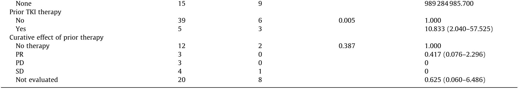
The P value and odds ratio (OR) are analyzed by univariate LR.
EC: etoposide and carboplatin; GC: gemcitabine and cisplatin; AC: pemetrexed and carboplatin; PR: partial response; PD: progressive disease; SD: stable disease; CI: confidence interval; T stage: size or direct extent of the primary tumor; N stage: degree of spread to regional lymph nodes; M stage: presence of distant metastasis; TNM stage: tumor, node, metastasis (TNM) staging classification according to the American Joint Committee on Cancer (AJCC).
3.2.2. Multivariable selection in all 53 examples
LR based on the AIC. To balance predictive model performance and complexity, we performed stepwise model selection by calculating the AIC. According to univariable analysis, there were ten potential predictive features. Fig. 2(a) shows the AIC values of each step in the backward stepwise LR, where ten predictive features were deleted one by one until the AIC no longer decreased. In general, models excluding the number of driver genes presented the worst AIC, which indicated that the number of driver genes was an important predictor. Moreover, the best multivariable model selected by the AIC was a five-variable LR model that included age, the number of driver gene mutations, type of prior chemotherapy, prior TKI therapy, and the source of the sample.
LASSO-LR. We performed LASSO regularization in LR to improve the predictive accuracy and interpretability. Here, we input ten significant features from the univariable LR model into a multivariable LASSO-LR. Two features of the ten features— namely, EGFR mutations and the number of driver genes—were screened out via LASSO-LR combined with 10-fold crossvalidation, where the optimal penalization coefficient was valued as one standard error (Figs. 2(b) and (c)).
《Fig. 2》

Fig. 2. Feature selection based on the lowest AIC and LASSO. (a) AIC for all possible models in the stepwise multivariable LR. A lower AIC indicates a better fit. Results are presented in columns defined by the number of variables in the model. In general, the model excluding the number of driver gene mutations achieved the worst AIC, while the model containing age, the number of driver gene mutations, type of prior chemotherapy, prior TKI therapy, and source of the sample was the one with the lowest AIC among all potential models. The upper abscissa is the number of non-zero coefficients in the model at this time. (b) Factor selection using the LASSO-LR model. was the optimal penalization coefficient. Binomial deviance was plotted versus lg(). Dotted vertical lines were plotted at the optimal values based on the minimum criteria and one standard error of the minimum criteria. The left vertical line represents the minimum error, and the right vertical line represents the cross-validated error within one standard error of the minimum. The optimal value of 1 standard error of the minimum was selected. The upper abscissa is the number of non-zero coefficients in the model at this time. (c) LASSO coefficients of ten candidate variables that are significant in univariable LR. The right dotted vertical line was plotted at one standard error of the minimum, resulting in two non-zero coefficients: the number of driver gene mutations and EGFR gene mutations.
《3.3. Model 2: SVM-RFE》
3.3. Model 2: SVM-RFE
SVM-RFE begins with a complete feature set and eliminates the least important feature for classification in each iteration according to the weight vector of the dimension length. According to the ranking of feature importance, which is visualized in Fig. 3(a), we first deleted the seven least important variables and then eliminated the remaining ten variables one by one to optimize the predictive accuracy. According to the mean predictive accuracy and the F1 score in the testing groups, the SVM-RFE model that included eight variables maintained the best performance with the least complexity (Figs. 3(b) and (c)). As a result, the eightfeature SVM-RFE was the best model among all the SVM classifiers.
《3.4. Model 3: GBDT》
3.4. Model 3: GBDT
To implement a GBDT, we used two commonly used algorithms: XGBoost and CatBoost. A large number of experiments indicated that multicollinearity among features did not hinder predictive classifications of decision trees [25]. Therefore, we input all 17 features in XGBoost and CatBoost in this study. The rank of features based on the XGBoost and CatBoost classification algorithms is also presented in Fig. 3(a). The representative structure of a decision tree generated by XGBoost and CatBoost is shown in Fig. 3(d).
《Fig. 3》
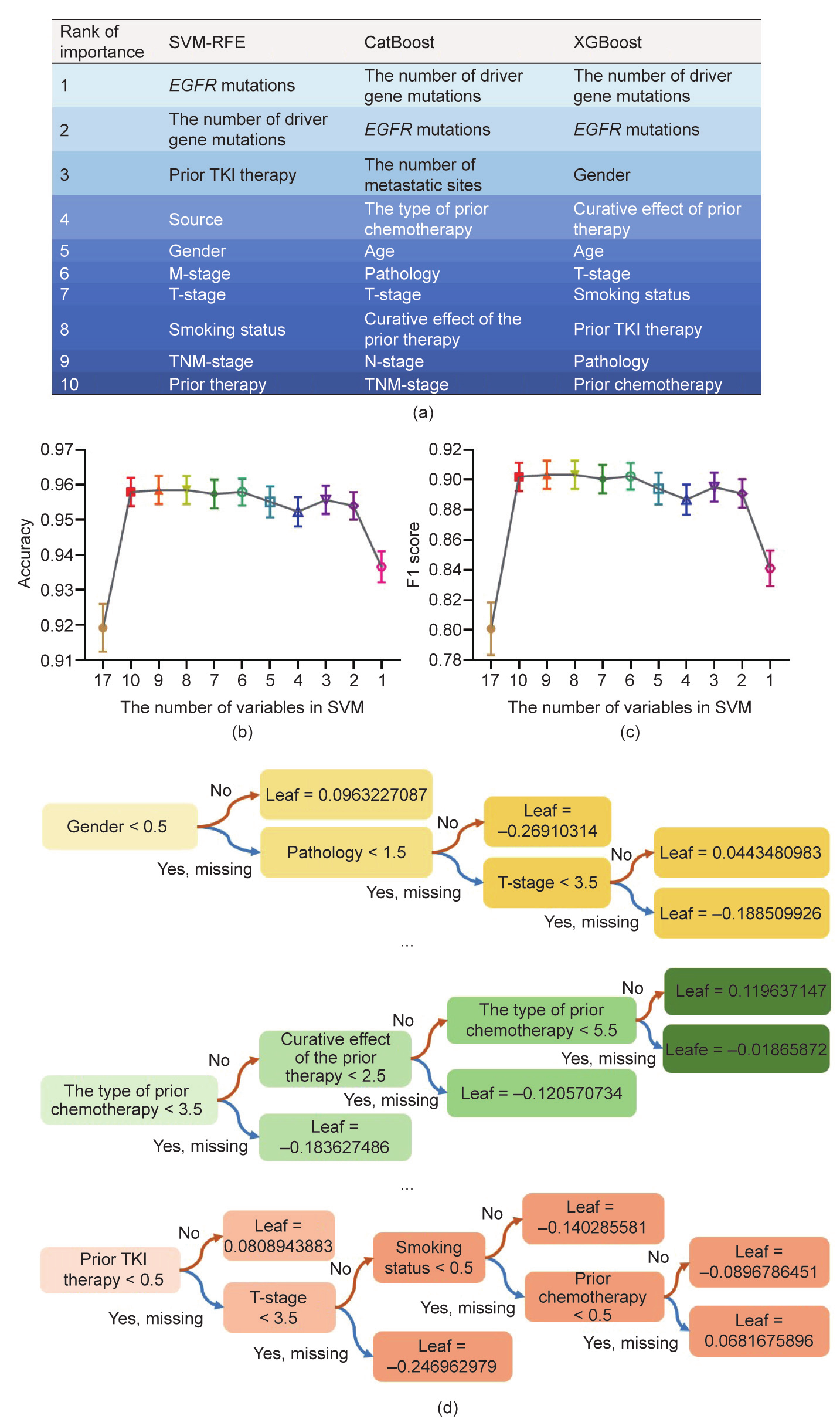
Fig. 3. Rank of importance of the top ten variables and the modeling process of the SVM-RFE and GBDT. (a) A chart showing the ten most critical variables according to three algorithms (SVM-RFE, CatBoost, and XGBoost), where the same color represents the same ranking. (b) The mean predictive accuracy of the SVM-RFE based on the different number of variables in 100 testing groups. The eight-feature SVM-RFE showed the highest accuracy with the fewest variables. (c) The mean F1 score of the SVM-RFE is based on the different number of variables in 100 testing groups. The eight-feature SVM-RFE exhibited the highest F1 score with the fewest variables. (d) A figure showing three out of 100 classification and regression trees (CARTs) obtained by XGBoost model training. After inputting the test sample into each CART, each sample’s predicted score can be obtained at the leaf node. After weighing the total score of 100 trees, each sample’s overall score and the corresponding classification can be obtained.
《3.5. Modeling in training groups and evaluating performance in testing groups》
3.5. Modeling in training groups and evaluating performance in testing groups
3.5.1. Comparison of different models
According to the AUC, accuracy, and F1 score of the 100 testing groups, CatBoost (mean accuracy = 0.960; mean AUC = 0.939; mean F1 score = 0.908) and the eight-feature SVM-RFE (mean accuracy = 0.950; mean AUC = 0.934; mean F1 score = 0.903) were dramatically better than the other three models, XGBoost (mean accuracy = 0.951; mean AUC = 0.908; mean F1 score = 0.873), LASSO-LR (mean accuracy = 0.937; mean AUC = 0.886; mean F1 score = 0.841), and LR based on the AIC (mean accuracy = 0.923; mean AUC = 0.850; mean F1 score = 0.789). Although the accuracies of the eight-feature SVM-RFE and XGBoost were statistically equal, CatBoost and the eight-feature SVM-RFE had the overall best performance. In addition, the mean accuracy (P = 0.103), AUC (P = 0.066), and F1 score (P = 0.128) of CatBoost and the eightfeature SVM-RFE were not significantly different (Fig. 4(a)), which showed promise in overcoming the limitations of the imbalanced, small sample dataset. We also evaluated the bias of the performance of these models (Fig. 4(b)), where the difference in accuracy, F1 score, and AUC between the training and testing groups remained below 8% except for the F1 score of LR based on the AIC (the difference between training and testing groups: 11.6%).
《Fig. 4》

Fig. 4. Comparison of the performance among different models. (a) The performance of single models. According to the predictive accuracy, the AUC, and the F1 score in 100 testing groups, CatBoost and the eight-feature SVM-RFE exhibited better performance than XGBoost, LASSO-LR, and LR based on the lowest AIC. (b) The bias of the model performance in the training groups and testing groups. *P < 0.05, **P < 0.01, ***P < 0.001, based on the paired-sample t-test between CatBoost and other models.
3.5.2. Improvement of model performance with the SMOTE
The SMOTE is an oversampling method that increases the number of positive classes through random data replication so that the positive and negative classes have equal numbers [26]. Herein, we applied the SMOTE to add ten more positive samples into training groups in order to accomplish feature selection, establish each model, and then test the models in the original 100 testing groups (Tables S2 and S3 in Appendix A). LASSO-LR had the same two features in the balanced training data applied with the SMOTE: EGFR mutations and the number of driver gene mutations. In comparison, LR based on the AIC selected the following seven features out of all the features: sex, EGFR mutations, number of driver gene mutations, M-stage, number of metastatic sites, type of prior chemotherapy, prior TKI therapy, and source of the sample. The rank of the ten most essential features in SVM-RFE, XGBoost, and CatBoost is shown in Fig. 5, with the number of driver gene mutations and EGFR mutations remaining as the leading contributors.
《Fig. 5》

Fig. 5. A chart showing the ten most critical variables according to three algorithms (SVM-RFE, CatBoost, and XGBoost) with SMOTE, where the same color represents the same ranking.
Interestingly, performing the SMOTE enhanced the overall efficacy of LASSO-LR (accuracy: 0.957 vs 0.923; AUC: 0.936 vs 0.850; F1 score: 0.902 vs 0.789; all P < 0.001), LR based on the AIC (accuracy: 0.945 vs 0.937; AUC: 0.904 vs 0.885; F1 score: 0.864 vs 0.841; all P < 0.001), the eight-feature SVM-RFE (accuracy: 0.961 vs 0.958, P = 0.025; AUC: 0.940 vs 0.935, P = 0.045; F1 score: 0.909 vs 0.903, P = 0.047), and XGBoost (accuracy: 0.934 vs 0.908, P = 0.004; AUC: 0.953 vs 0.952, P = 0.630; F1 score: 0.896 vs 0.874, P = 0.108) (Figs. 6(a)–(d)). However, the application of the SMOTE did not impact the predictive ability of CatBoost for genotype mismatching (accuracy: 0.961 vs 0.960; AUC: 0.909 vs 0.908; F1 score: 0.940 vs 0.939; all P > 0.05) (Fig. 6(e)).
In this case, CatBoost demonstrated the same stable potential for both even and uneven samples. However, LR achieved the largest significant performance enhancement with the SMOTE, which revealed that LR should be recommended for even data. Moreover, we described an approach that can improve the SVM-RFE and XGBoost in small, uneven samples.
3.5.3. Ultimate optimization of the ensemble classifier for performance
Considering the dramatic enhancement of the performance of most models after applying the SMOTE, we finally used an ensemble classifier after conducting the SMOTE based on LR based on the AIC, the eight-feature SVM-RFE, XGBoost, and CatBoost. Surprisingly, the accuracy (mean = 0.975), AUC (mean = 0.949), and F1 score (mean = 0.938) of the ensemble classifier were further optimized compared with those of the single model (Fig. 6(f)). Moreover, the bias of the ensemble classifier in the training and testing groups was also superior (all differences below 5%) (Fig. 6(f)).
Therefore, we propose an ensemble classifier based on single optimized models, which overcame the sample size and distribution defects and achieved the best level of discrimination and stability.
《Fig. 6》

Fig. 6. The performance of SMOTE with different algorithms. (a) The performance of the introduction of SMOTE to LASSO-LR. (b) The performance of the introduction of SMOTE to LR based on the AIC. (c) The performance of the introduction of SMOTE to eight-feature SVM-RFE. (d) The performance of the introduction of SMOTE to CatBoost. (e) The performance of the introduction of SMOTE to XGBoost. (f) The performance of the ensemble classifier in training and testing groups by conducting the SMOTE based on LR based on the AIC, the eight-feature SVM-RFE, XGBoost, and CatBoost. *P < 0.05, **P < 0.01, ***P < 0.001, based on the paired-sample t-test.
《4. Discussion and conclusion》
4. Discussion and conclusion
This study initially developed a predictive model for driver gene mutation inconsistency between NOG/PDX models and patient samples. A total of 53 lung cancer NOG/PDX models were successfully engrafted and excised, including 42 NOG/PDX models with driver gene mutations that matched those in parental tumors and 11 NOG/PDX models with nonmatching tumors. To analyze this small unbalanced database, we used five algorithms: LR based on the AIC, LASSO-LR, eight-feature SVM-RFE, XGBoost, and CatBoost. According to the indexes in the testing groups, CatBoost and eight-feature SVM-RFE had the best performance. Moreover, use of the SMOTE generally improved the performance of all models except CatBoost at the fundamental level. In the end, the ensemble classifier based on single models had the best performance (mean accuracy = 0.975; mean AUC = 0.949; mean F1 score = 0.938), with an acceptable bias between the training and testing groups (all differences under 5%).
The generation and passaging of PDX models are dynamic events in which clonal and subclonal alterations frequently occur, especially when the development of P1 PDX models is slow, which gives adequate time for tumor cells to mutate and adapt to a new environment [27,28]. In addition to cell-autonomous heterogeneity, stromal heterogeneity in the tumor microenvironment (TME) is a critical reason why driver genotypes of PDXs differ from those of parental tumors [12]. It has been reported that SCC is much more prone to tumorigenesis in nude mice than ADC [18], which is inconsistent with our conclusion that SCC is the most challenging tumor type to establish NOG/PDX models with genetic matching. More CD8+ TILs were detected in SCC tumors than in non-SCC cell nests [29], which suggests that PDX models of SCC may lose more tumor stroma during xenograft engraftment. Moreover, SCC has been found to be prone to carry significantly more clonal mutations than ADC [30], contributing to more clonal selection. Although age had a small weight in multivariable LR, we have not found an appropriate method to illustrate that a younger age rather than an older age is a risk factor for driver gene matching [31]. Most PDX models use 8-week-old mice rather than aged mice (> 8 months), while recent studies have found that aging could dramatically alter components of the TME [32]. Therefore, inconsistencies in the age of mice and patients could be a reason why age was found to be a predictive feature here. Another feature, the source, also played a negative role in genotype matching, which differed from tumor engraftment. Although fluid sources have been suggested to have a higher engraftment rate [33], we found it was more challenging to maintain driver genotypes of parental tumors in fluid-derived tumor xenografts.
The number of driver gene mutations, including clonal and subclonal mutations, is associated with intratumor heterogeneity, genomic instability, and chromosomal instability [34]. First, the largest coefficient of the driver gene number in the multivariable LR model also illustrates its importance in developing nonpatient-matched genotypes. Second, PDX models from EGFR mutant lung cancers were reported to have poor histological differentiation and frequent EGFR mutation loss [35], which supported the high risk of EGFR mutant inconsistency in NOG/PDX models in this study. Third, the evidence that pemetrexed increased the number of TILs and upregulated immune-related genes related to antigen presentation might support the conclusion that PDX models from patients receiving pemetrexed were less likely to maintain the original genotypes [36]. TKIs have been proven to alter the pulmonary TME, including increases in CD8+ T cells and mononuclear myeloid-derived suppressor cells (M-MDSCs; CD11b+ Ly6– G– - Ly6Chigh), and decreases in fewer Foxp3+ T regulatory cells (Tregs) and M2-like macrophages (CD206+ ) [37]. In addition, clonal selection is a frequent occurrence during TKI therapy, resulting in TKI resistance [38]. Interestingly, we found that factors that promoted TILs promoted genotype stability during NOG/PDX model establishment, which needs further verification (Fig. 7(a)).
Recently, ML has been a useful method for predictive modeling in numerous areas, as it enables predictive models to systematically ‘‘learn” information from initial data and adapt to each new data environment [39]. However, ML has not been widely used in small sample databases (less than ten frequencies per predictor variable), which is a common characteristic of biomedical animal models with high costs and complicated techniques [40]. Ultimately, the ML algorithms that we used to establish predictive tools for lung cancer NOG/PDX models had excellent performance, which not only provides a predictive tool to screen lung cancer patients for NOG/PDX models for precision immunotherapy, but also offers a general approach for building predictive models with small biomedical samples (Fig. 7(b)).
《Fig. 7》
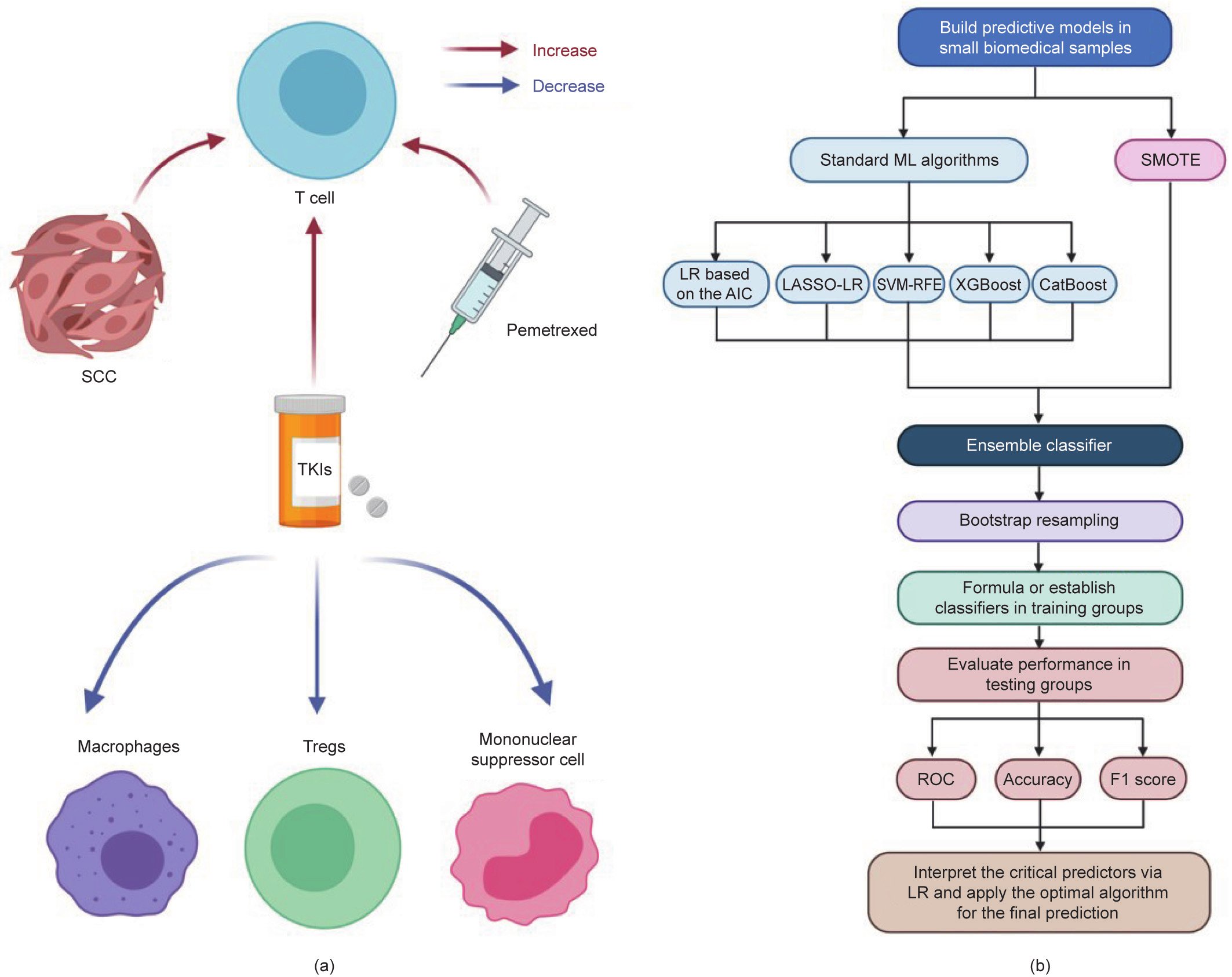
Fig. 7. Potential impact of the TME on driver gene mutations and a flow chart for building predictive models in small datasets. (a) Association between the factor contributing to the inconsistency of driver gene mutation and the TME. According to univariable and multivariable LR, SCC, application of pemetrexed, and prior TKIs therapy were risk factors for nonmatching genotypes between PDX models and parental tumors. All of these three factors raised TILs. Moreover, TKIs could decrease Foxp3+ Tregs, mononuclear myeloid-derived suppressor cells (CD11b+ Ly6– G– Ly6Chigh), and M2-like macrophages (CD206+ ) in the TME. (b) Flow chart for building predictive models in small biomedical datasets: ① When the dataset is uneven, perform SMOTE first. Select features to develop a multivariable model in all samples with standard ML algorithms, including stepwise LR based on the AIC, LASSO-LR, SVM-RFE, XGBoost, CatBoost, and so forth. ② Propose an ensemble classifier based on the optimized single models. ③ Perform bootstrap resampling to avoid overfitting and achieve stable performance. ④ Formulate the predictive score or establish the predictive classifier in training groups. ⑤ Evaluate the predictive model based on the ROC, accuracy, and F1 score in the corresponding testing groups to determine an optimal algorithm for modeling. ⑥ Interpret the critical predictors for the positive class by LR, and apply the optimal algorithm for the final prediction.
Several limitations remain in this study. First, the number of patients included in the study was limited, and larger scale experiments should be carried out to further validate these conclusions. Second, the prediction results of this model cannot be accurate to each driving gene mutation due to the limited training data. Third, the EGFR mutation status was both an independent variable and an outcome, which may cause collinearity. Last, potential selection bias was inevitable, and this study’s sex ratio was uneven. Larger scale trials should be performed to further validate these conclusions.
In conclusion, we established a predictive model for driver gene mutation inconsistency between NOG/PDX models and patient samples based on ML, which promises to improve the success rate of PDX establishment and reduce the massive economic loss. Furthermore, the NOG mice used in this study are considered to be an excellent choice for building PDX models for cancer immunotherapy, although they are not well studied. Therefore, the model we established has potential for immunotherapy screening and development.
《Acknowledgments》
Acknowledgments
Fig. 5 was created with BioRender.com. Language polishing was completed by a native editor from Springer Nature Author Services (SNAS).
This study was supported in part by a grant of National Natural Science Foundation of China (81802255); Clinical Research Project of Shanghai Pulmonary Hospital (FKLY20010); Young Talents in Shanghai (2019 QNBJ); ‘‘Dream Tutor” Outstanding Young Talents Program (fkyq1901); Clinical Research Project of Shanghai Pulmonary Hospital (FKLY20001); Respiratory Medicine, a key clinical specialty construction project in Shanghai, promotion and application of multidisciplinary collaboration system for pulmonary non infectious diseases; Clinical Research Project of Shanghai Pulmonary Hospital (fk18005); Key Discipline in 2019 (Oncology); Project of Shanghai Municipal Health Commission (201940192); Scientific Research Project of Shanghai Pulmonary Hospital (fkcx1903); Shanghai Municipal Commission of Health and Family Planning (2017YQ050); Innovation Training Project of SITP of Tongji University, Key Projects of Leading Talent (19411950300); and Youth project of hospital management research fund of Shanghai Hospital Association (Q1902037).
《Authors’ contributions》
Authors’ contributions
Yayi He, Xuzhen Tang, Junjie Zhu, and Yang Yang conceived the concepts of the research. Yayi He, Haoyue Guo, and Li Diao designed the research. Hui Qi and Chunlei Dai established PDX models. Haoyue Guo performed the image preprocessing. Haoyue Guo and Li Diao contributed to machine learning. All authors analyzed the data and wrote the paper.
《Compliance with ethics guidelines》
Compliance with ethics guidelines
Yayi He, Haoyue Guo Li Diao, Yu Chen, Junjie Zhu, Hiran C. Fernando, Diego Gonzalez Rivas, Hui Qi, Chunlei Dai, Xuzhen Tang, Jun Zhu, Jiawei Dai, Kan He, Dan Chan, and Yang Yang declare that they have no conflict of interest or financial conflicts to disclose.
《Appendix A. Supplementary data》
Appendix A. Supplementary data
Supplementary data to this article can be found online at https://doi.org/10.1016/j.eng.2021.06.017.


 京公网安备 11010502051620号


