
《1. Introduction》
1. Introduction
Since the discovery of well-defined orbital angular momentum (OAM) [1], beams carrying OAM proved to be an important tool in the ascension of photonics. Characterized by the presence of an azimuthal phase eimθ , where the index m is known as topological charge and θ is the azimuthal angle [2], OAM beams are poised to enable a number of applications, including information transfer [3], optical tweezers [4,5], quantum teleportation [6], and computation [7]. Light possessing an OAM, also known as an optical vortex, usually possesses a ring-like intensity distribution, whereas its topological charge can be measured by a number of optical techniques, such as interferometry [8], diffraction through a slit [9–11], and the tilted-lens method [12], to cite a few.
One of the most common ways of generating optical vortices in a laboratory would be using a spatial light modulator (SLM) [13,14]. This liquid-crystal-based device allows one to use such a computer-generated phase-mask as a hologram, which makes it quite simple to generate any sort of optical beam. Other options include so-called spiral phase plates (SPPs) [15,16] and q-plates— where the latter is another type of liquid crystal device with inhomogeneous patterned distribution of the local optical axis in the transverse plane [17,18]. However, in the domain of integrated optics, compact devices that can readily be integrated on a chip are needed in order to create optical beams carrying OAM. To address this need, the most recently proposed approach to generate optical vortices relies on metasurfaces, including both dielectric [19] and plasmonic [20,21] structures.
Although most commonly used optical vortices are known to be ring-shaped, there are other groups of beams with different shapes that also carry an OAM. Bessel beams (BBs), which are characterized by an intensity distribution consisting of an infinite multiring pattern, is one of these groups [22,23]. BBs are particularly interesting because of their self-healing property [24–26]. Moreover, higher-order BBs find applications for particle trapping [27,28] and imaging systems [29,30]. Considering other symmetries, elliptical vortices (EVs) are another group of beams possessing OAM. First studied by Bandres and Gutiérrez-Vega [31,32] and Schwarz et al. [33], Ince–Gaussian (IG) beams were found by solving the free-space paraxial wave equation in elliptical coordinates. IG beams can be related to either Laguerre–Gaussian (LG) and Hermite–Gaussian (HG) beams by changing their eccentricity parameter to 0 and  respectively. On the other hand, EVs can be found by performing a change of variables in the LG mode [34]. Introducing the elliptical parameter η, which assumes values between 0 and 1, simplifies analytical studies of EVs. The elliptical analogue for BBs is the Mathieu beams (MBs), whose intensity profiles consist of an infinite number of concentric ellipses [35]. It is important to mention that exact BBs and MBs, strictly speaking, cannot be realized in the laboratory experiment due to their infinite transverse profile implying an infinite energy requirement. Nevertheless, truncated BBs and MBs can be generated and studied experimentally [36,37].
A new group of asymmetrical beams was recently developed using an acousto-optical deflector (AOD) together with log-polar optics to generate higher-order Bessel beams integrated in time (HOBBIT) [38,39]. This method enables the generation of rapidly tunable OAM beams, which reach switching speeds of up to tens of megahertz with a sub-microsecond response time and highpower laser systems, due to the AOD’s very high damage threshold. Such properties make HOBBITs suitable to probe turbulence by rapidly scanning OAM states along an optical path [40] and may be helpful in communication protocols that demand fastswitching OAM modes and high power levels.
One of the most fascinating research directions in the field of optical vortices is the study of such structured light–matter interactions in various linear and nonlinear media. In particular, nonlinear processes such as second-harmonic generation [41], optical Kerr effect [42,43], self-focusing [44,45], and optical-parametric oscillations [46] have been reconsidered in the presence of OAM beams. Moreover, rapid progress in nanophotonics opened up new ways of ‘‘engineering” the nonlinear medium itself in order to tailor many of these nonlinear light–matter interactions, including self-focusing, modulation instability (MI), and spatial soliton formation [47]. A stability analysis of these solitons can be realized by using a variational approach together with a perturbation method [48]. In particular, carefully engineered nanocolloidal suspensions facilitate new ways of tailoring linear and nonlinear propagation. Indeed, it was shown that liquid suspensions of spherical dielectric nanoparticles can exhibit very large optical nonlinearities [47]. The nonlinearity of nanoparticle suspensions originates from the fact that in the presence of a continuous wave, optical field dielectric nanoparticles experience an optical dipole force proportional to the particle polarizability in the liquid. In the case of particles of higher refractive index np than the surrounding liquid nb, the polarizability is positive and the particles experience an electrostrictive volume force that attracts them into the spatial regions of high intensity thus increasing the local density and the local refractive-index. If optical vortices are considered, it has been predicted and experimentally demonstrated that an azimuthal MI may lead to different regimes of nonlinear beam shaping depending on the properties of the medium and the initial parameters of the OAM beam. In particular, a so-called necklace beam (NB) [49– 51] formation has been demonstrated.
A majority of previous studies on nonlinear light–matter interactions in colloidal suspensions focused on symmetric OAM beams, including the formation of NBs originating from symmetric optical vortices [49,51]. The dynamics of those NBs were also studied, focusing on a deeper discussion about stability, trajectories, and the formation of new optical beam structures [50]. Here, we report the behavior of several families of complex-shaped OAM beams in negative-polarized nanocolloidal suspensions.
Our paper is structured as follows. In Section 2, we review various types of OAM beams, including LG beams, EV beams, and HOBBIT. In Section 3, we describe all-dielectric as well as plasmonic-particles-based engineered colloidal media with saturable nonlinearity. In Section 4, we perform linear stability analysis followed by full numerical simulations for each family of beams. Finally, in Section 5, we summarize the results of our studies of nonlinear OAM beam propagation in saturable nonlinear nanocolloidal media.
《2. Optical beams carrying OAM》
2. Optical beams carrying OAM
《2.1. Laguerre–Gaussian modes》
2.1. Laguerre–Gaussian modes
Let us consider the orthogonal set of OAM-carrying beams defined by LG modes, which are characterized by the indices p and m, which respectively refer to the radial order and topological charge. For the case where p = 0, these optical modes can be written as [1,2]
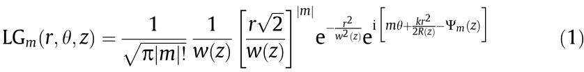
where  is the beam width,
 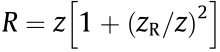 is the wavefront radius of curvature,
 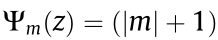 arctan (z/zR) is the Gouy phase, and zR is the Rayleigh range. This set of optical modes is a family of solutions to the Helmholtz equation under the paraxial approximation in cylindrical coordinates and Fig. 1 shows the intensity distribution for some values of m. If one is specifically interested in studying the behavior, interaction, or characterization of the OAM, it is common to consider z = 0 and work with the mth order optical vortex [49]:
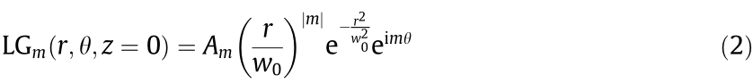
Other beams that can also carry an OAM include higher-order Bessel [52] and circular Airy beams [53], which constitute the solutions of the Helmholtz equation in cylindrical coordinates and the paraxial wave equation, respectively.
《Fig. 1》
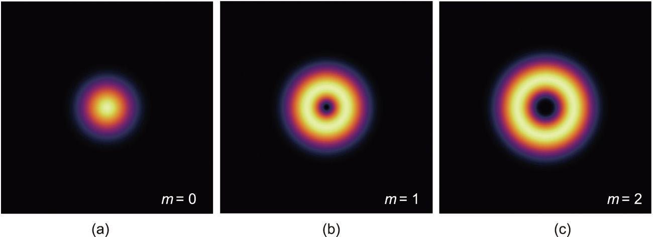
Fig. 1. Intensity distribution for LG modes with topological charges (a) m = 0, (b) m = 1, and (c) m = 2.
《2.2. Elliptical vortices》
2.2. Elliptical vortices
From an experimental standpoint, it has been shown that elliptic beams can be generated using an oblique incidence of an axially symmetric beam onto an optical element such as a conical axicon or a binary diffractive axicon [54,55]. From a theoretical viewpoint, exact solutions of the Helmholtz equation can be obtained for the MBs [35], which possess self-healing properties similar to that of the BBs. On the other hand, under the paraxial approximation, the IG modes arise as a family of solutions [31]. Their eccentricity parameter ε adjusts the ellipticity of the transverse structure of the beam, in which the transition to an LG (HG) mode occurs when ε tends to zero (infinite). Even though these are well-behaved solutions, they are not easily handled analytically. For this reason, alternative methods of generating EVs were developed. It was demonstrated that, by just adding an ellipticity parameter η (0 ≤η ≤1), we have the following expression for an mth order elliptical optical vortex [34]:
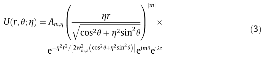
where Am,η denotes the amplitude,  is the beam width, and
  is the propagation constant. By making use of the elliptical coordinates in Eq. (3), where
 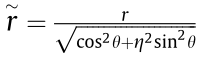 and
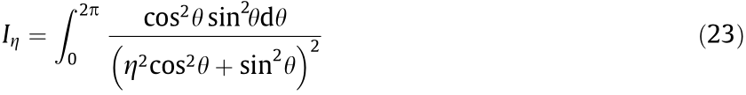
and 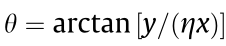 , the angular dependence of the radial variable is explicitly displayed. Fig. 2 shows the intensity distribution of EVs for various ellipticity parameters η. Due to the similarity to regular cylindrical optical vortices, one can make use of this approach to analytically study optical effects as the cylindrical symmetry is broken into an elliptical symmetry.
《Fig. 2》
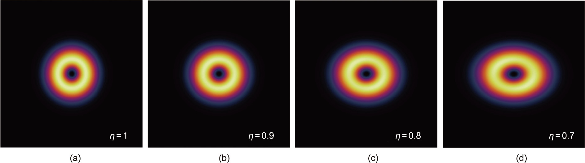
Fig. 2. Intensity distributions for EVs with topological charge m = 1 and ellipticity parameter (a) η = 1, (b) η = 0.9, (c) η = 0.8, and (d) η = 0.7.
《2.3. Higher-order Bessel beams integrated in time》
2.3. Higher-order Bessel beams integrated in time
The HOBBIT system consists of a series of optical devices designed to prepare the input beam impinging on a pair of logpolar optical elements. It converts each Gaussian beam in an array to an asymmetric higher-order Bessel–Gaussian beam after multiple transformations. This results in a superposition of copropagating higher-order Bessel–Gaussian beams possessing OAM. This technique may be useful to multiple applications, including quantum communication protocols, beam shaping, filamentation, and sensing methods for atmospheric turbulence and underwater systems.
The near-field output of a HOBBIT system with topological charge m at z = 0 can be expressed as [38–40]

where r0 controls the ring radius, β is the asymmetry parameter, and  is the amplitude. This leads to an asymmetric ringshaped beam, where the asymmetry is controlled by β. Fig. 3 [38] shows the amplitude distribution as well as the phase pattern for HOBBITs with the topological charges m = ±3, ±1.2, and 0. As reported in Ref. [38], the efficiency of the AOD coupled with the log-polar system is up to 60%. This means that, for an input power of 30 W, the output would be approximately 18 W.
《Fig. 3》
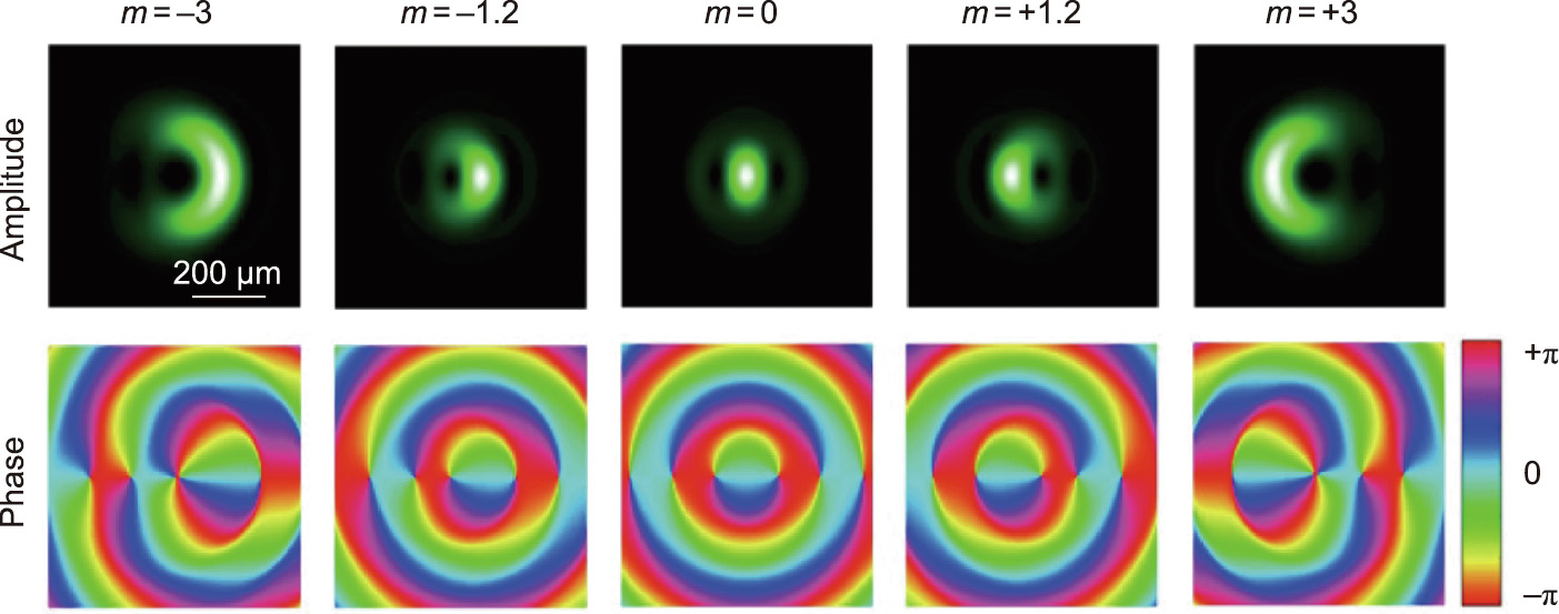
Fig. 3. Amplitude and phase distribution of HOBBITs for the topological charges m = ±3, ±1.2, and 0. Here, β = 0.66, = 329 μm, and r0 = 850 μm. Reproduced from Ref. [38] with permission.
《3. Saturable nonlinear media》
3. Saturable nonlinear media
《3.1. Self-focusing saturable nonlinearity》
3.1. Self-focusing saturable nonlinearity
Initially, saturable nonlinearities were introduced as a correction to the cubic Schrödinger equation (CSE), which is a generic equation describing slow-varying envelopes in conservative, dispersive systems [56]. Optical fields interacting with such systems are governed by the normalized equation [57,58]:

where 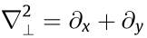 is the Laplacian and
  is the function related to the nonlinear response of the system. For instance, selffocusing saturable nonlinearity can be modeled by
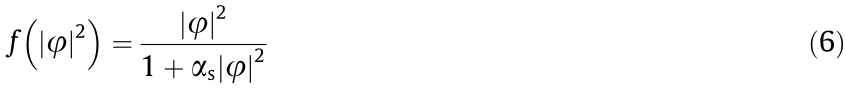
where αs is the saturation parameter. Notice that, for αs = 0, the Kerr limit is achieved. Through this approach, it was demonstrated the existence of soliton solutions carrying OAM [57], the self-trapping effect [58], and NBs [59], among other findings. In Fig. 4, the authors demonstrate the azimuthal instability development in solitons carrying OAM propagating in a saturable self-focusing medium [57].
《Fig. 4》
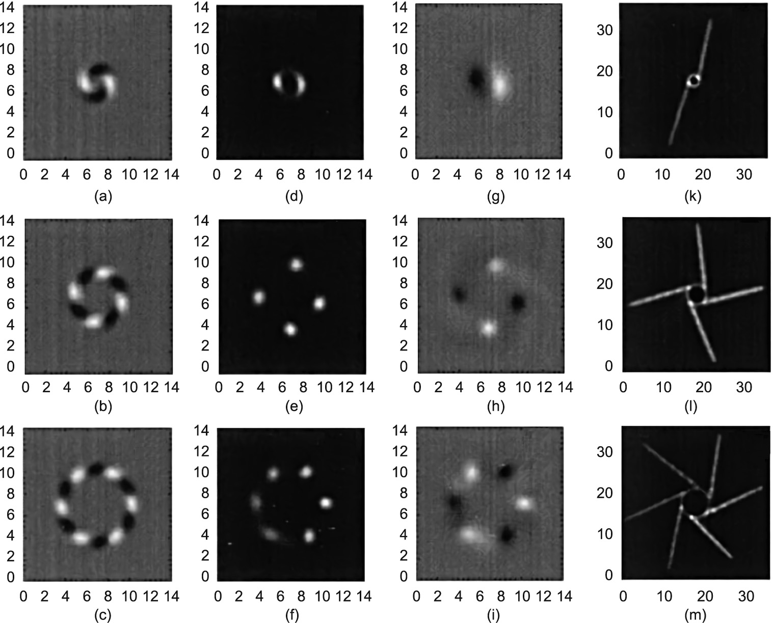
Fig. 4. Azimuthal modulational instability development and soliton trajectories with input topological charges (top)  = 1, (middle) = 2, and (bottom) = 3. Here, the values for the saturation parameter and propagation constant are, respectively, α = 0.1 and κ= 1. (a–c) Real part of the perturbed field possessing maximal growth rate; (d–f) numerical calculations of the optical intensities where the solitons have already developed; (g–i) real part of the electric field at the same point, highlighting the phase difference between the solitons; (k–m) superimposed transverse intensities at different propagation positions. Reproduced from Ref. [57] with permission.
《3.2. Engineered colloidal suspensions》
3.2. Engineered colloidal suspensions
The nonlinear response of nanoparticle suspensions was first studied by El-Ganainy et al. [47] in 2007. Starting from the particle current continuity equation  one can make use of the Nernst–Planck equation and obtain the expression for the particle current density [47,60]:

where the diffusion coefficient is denoted by D, the particle convective velocity by v, and the particle concentration by ρ. Here, v is related to the optical force F acting on the nanoparticles as v = μF, where μ is the particle’s mobility. In this model, particle–particle interactions are neglected and highly diluted mixtures are assumed. After combining these expressions, we get the Smoluchowski equation [47,60]:

Now, some assumptions are needed in order to solve this equation. First, let us consider steady-state solutions ( = 0). Second, with the system under equilibrium, diffusion (J = 0) is the responsible to balance the particle’s movement. Finally, if we consider the Rayleigh regime (wavelength is large compared to the particle aspect ratio), the external optical force can be obtained within the dipole approximation and is expressed as
  where I =
  is the light intensity and α is the particle polarizability [47]. Still under the dipole approximation, one can express the polarizability of a spherical particle with refractive index np as [47,61]

where Vp is the volume of the particle, ε0 is the permittivity in freespace, and mr = np/nb is the ratio of the particle’s refractive index np to the refractive index of the background nb. Notice that, if mr > 1 (mr < 1), the polarizability is positive (negative). After solving Eq. (8) and making use of the Maxwell–Garnett formula, one can find the local index change [47,61,62]. In a relatively small index contrast regime (|mr < 1|), we find the optical nonlinearity of the nanosuspensions to be [47]

The scattering losses can also be included into the system. Under the Rayleigh regime, the scattering cross section can be written as
with  representing the particle radius. Now, we can obtain the components to write the beam evolution equation through a nanosuspension system. After modifying the Helmholtz equation,
  where
where  the nonlinear Schrödinger equation (NLSE) for this system reads [47]

Here, for either positive or negative polarizabilities, the nonlinear response is self-focusing. For the positive case, the refractive index of the particle is higher than the background (np > nb), leading the particles to move toward the light and increasing the scattering losses. On the other hand, negative polarizability regimes (np < nb) make the particles to move outward from the beam, reducing the scattering losses and leading to a more stable propagation through the system. Fig. 5 shows a sketch of the particle dynamics for a nanosuspension system with both positive and negative polarizability [47].
《Fig. 5》

Fig. 5. Nanoparticle dynamics under interaction with a highly intense beam for (a) positive and (b) negative polarizabilities. Reproduced from Ref. [47] with permission.
《3.3. Plasmonic suspensions》
3.3. Plasmonic suspensions
In the case of the all-dielectric-based saturable nonlinear media described above, high power illumination was usually required to ignite the nonlinear response. However, replacing the dielectric nanoparticles with metallic ones allows relaxing this requirement for the input powers of continuous-wave (CW) lasers [63]. Using various metallic structures, including gold nanorods, silica–gold nanoshells, and gold and silver spheres, the authors of Ref. [63] demonstrate that the nonlinear dynamics are governed by thermal responses, scattering, and optical forces acting on the particles. For this system, the NLSE can be extended by including the thermal effects and, after some algebra, it can be written as [63]
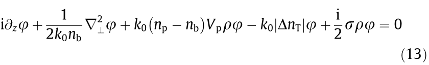
where ρ is the particle concentration and  is the refractive index change mediated by the thermal effects. Here, the interplay between thermal effects and nonlinear colloidal responses leads to a nonlinearity compared to cubic–quintic saturable nonlinear media
In Ref. [63], the authors experimentally demonstrate a selftrapping behavior in Gaussian beams propagating in both positive and negative metallic nanosuspensions. Fig. 6 presents the beam self-trapping in a negative polarizability nanosuspension system composed of gold nanorods, while Fig. 7 displays the interactions within positive polarizability media filled with gold (Figs. 7(a)– (d)) and silver (Figs. 7(e)–(h)) particles [63].
《Fig. 6》
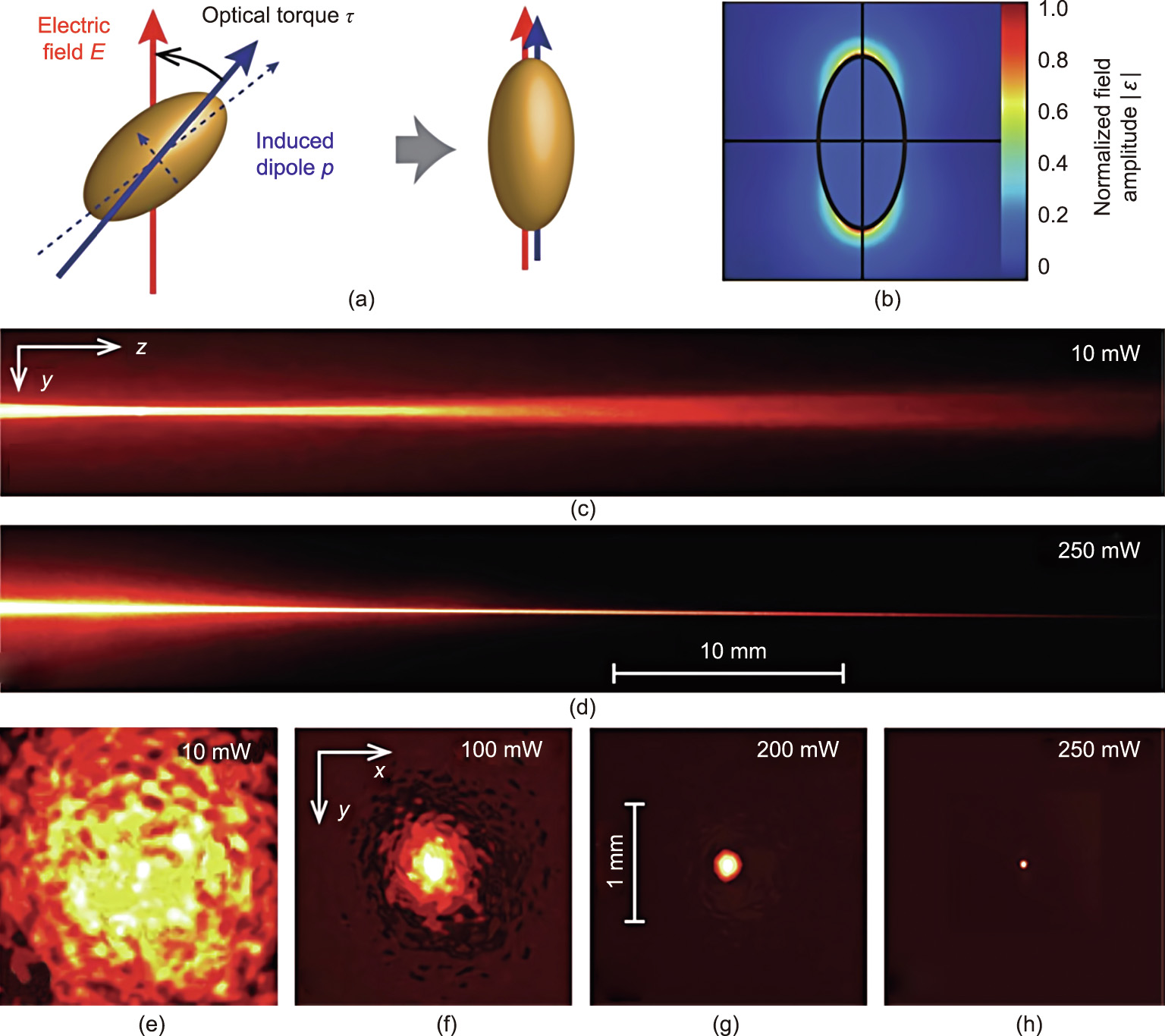
Fig. 6. (a) Orientation of gold nanorods, where major and minor diameters are 100 and 50 nm, respectively, under the presence of a linearly polarized electric field. (b) Normalized field amplitude surrounding the nanorod at the longitudinal plasmon resonance. (c) Propagation of a low-power beam (10 mW) in an aqueous solution with suspended gold nanorods. (d) Stable filamentation formation at 250 mW upon 5 cm propagation in a negative polarizability colloidal solution. (e–h) Transverse beam profiles with various input power after propagation (5 cm), highlighting the self-trapping effect as the power level grows. The output profiles have been normalized respectively to their maximum intensities. Reproduced from Ref. [63] with permission.
《Fig. 7》

Fig. 7. (a) Normalized field amplitude of 40 nm gold spheres in their surrounding at the plasmon resonance; (b) optical propagation at 10 mW; (c) self-trapping of positive polarizability suspensions at 150 mW induced by thermal effect; (d) thermally induced nonlinear defocusing with 500 mW. (e) Normalized field amplitude of 100 nm silver spheres in their surrounding at the plasmon resonance; (f) collapsing at 10 mW with positive polarizability suspensions; (g) at 2000 mW, thermal effects start balance the positive polarizability nonlinear effects, stabilizing the beam; (h) eventually, thermal effects dominate the self-focusing nonlinearity. Reproduced from Ref. [63] with permission.
《4. Azimuthal modulational instability》
4. Azimuthal modulational instability
《4.1. NB generation in circular optical vortices》
4.1. NB generation in circular optical vortices
Now, let us introduce the theoretical model used to study the modulational instabilities of optical vortices propagating in colloidal media. One can normalize Eq. (12) by introducing a few parameters 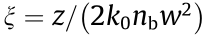 , X = x/w, Y = y/w, and w–2 =
  After substitution, Eq. (12) reads

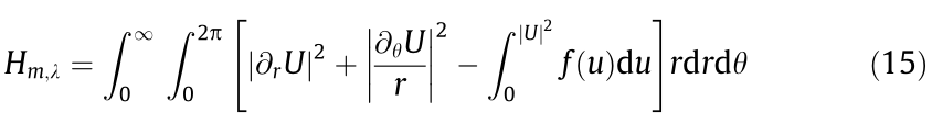
where U is the normalized field amplitude, δ is the loss coefficient, and ξ is the normalized longitudinal axis. Here,  =1 ( = 1) refers to a positive (negative) polarizability case. By making use of a variational method approach [48], one can analytically derive the expressions for the beam width () and beam amplitude () for a given topological charge m. After reducing the system to a (2 + 1) dimensional problem, the Hamiltonian for the lossless case is expressed as
and the power integral as

Here, the nonlinear term is  . Since Eqs. (3) and (4) are invariants for the NLSE, we can solve the variational problem
  = 0, where
  is the action integral, in order to determine and . Let us consider perturbations along the mean radius
  and the amplitude
 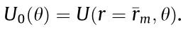 For the circular optical vortex case, the perturbed solution can be expressed as

where  is the unperturbed field and
  with j = 1, 2, is the perturbed amplitude
  The topological charge indices m and M and the propagation constants
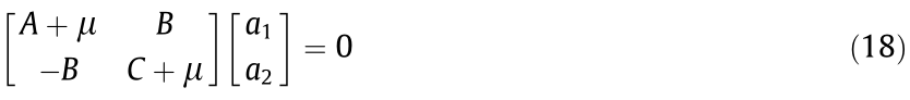
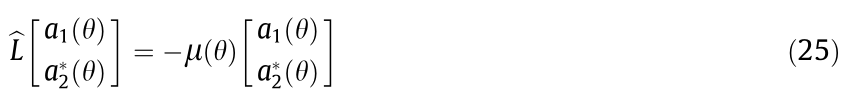
  and μ refer to the steady-state solutions and the perturbation, respectively. After linearizing Eq. (14) using the solution for Eq. (17), this leads to the eigenvalue problem:
with

Here,  and the derivative with respect to
  is denoted by the prime. This brings us to two expressions: one related to the propagation constant
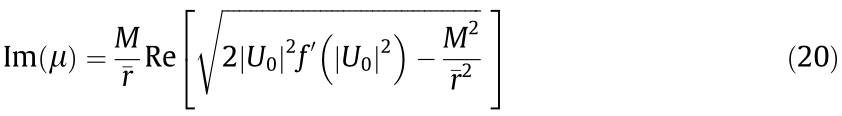
 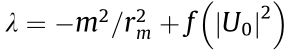 and the other for the correction of the propagation constant μ related to the MI. By taking the imaginary part of μ, we find the MI gain [47,64]:
After fixing the topological charge m, it was demonstrated in Ref. [49] that positive polarizability systems have higher MI gain than for the negative case. Refer to Fig. 8 for the gain curves Im(μ) as a function of the perturbation azimuthal index M for various topological charges [49]. This means that, for a fixed initial power, MI acts earlier as the beam propagates for positive polarizability than for negative polarizability. In other words, the system becomes more unstable for positive polarizability systems, as the particles move toward the light, increasing the scattering losses. In addition, the number of peaks in the NB is larger for positive polarizability than for the negative case. Figs. 9 and 10 show light propagation with various topological charges m through positive and negative polarizability nanosuspensions, respectively [49]. An experimental validation of these results using negative polarizability nanosuspensions was demonstrated in Ref. [51]. Fig. 11 shows the experimental formation of NBs using the initial topological charges m= 1, 2, and 4 [51].
《Fig. 8》
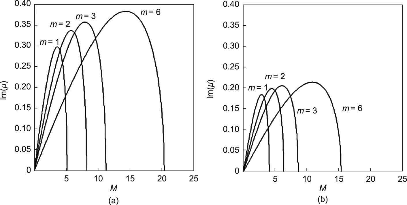
Fig. 8. MI gain as a function of the azimuthal perturbed index M for (a) positive and (b) negative polarizability suspensions for various initial topological charges m. Reproduced from Ref. [49] with permission.
《Fig. 9》
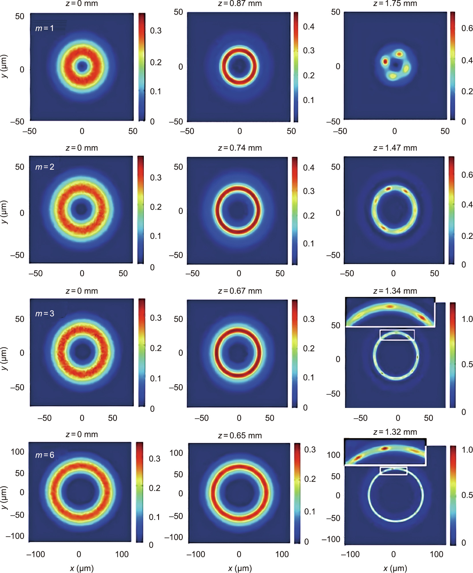
Fig. 9. Intensity distribution displaying the NB formation for initial topological charges m = 1, 2, 3, and 6 in a positive polarizability suspension. Details of the pointed region are shown in the insets. Reproduced from Ref. [49] with permission.
《Fig. 10》
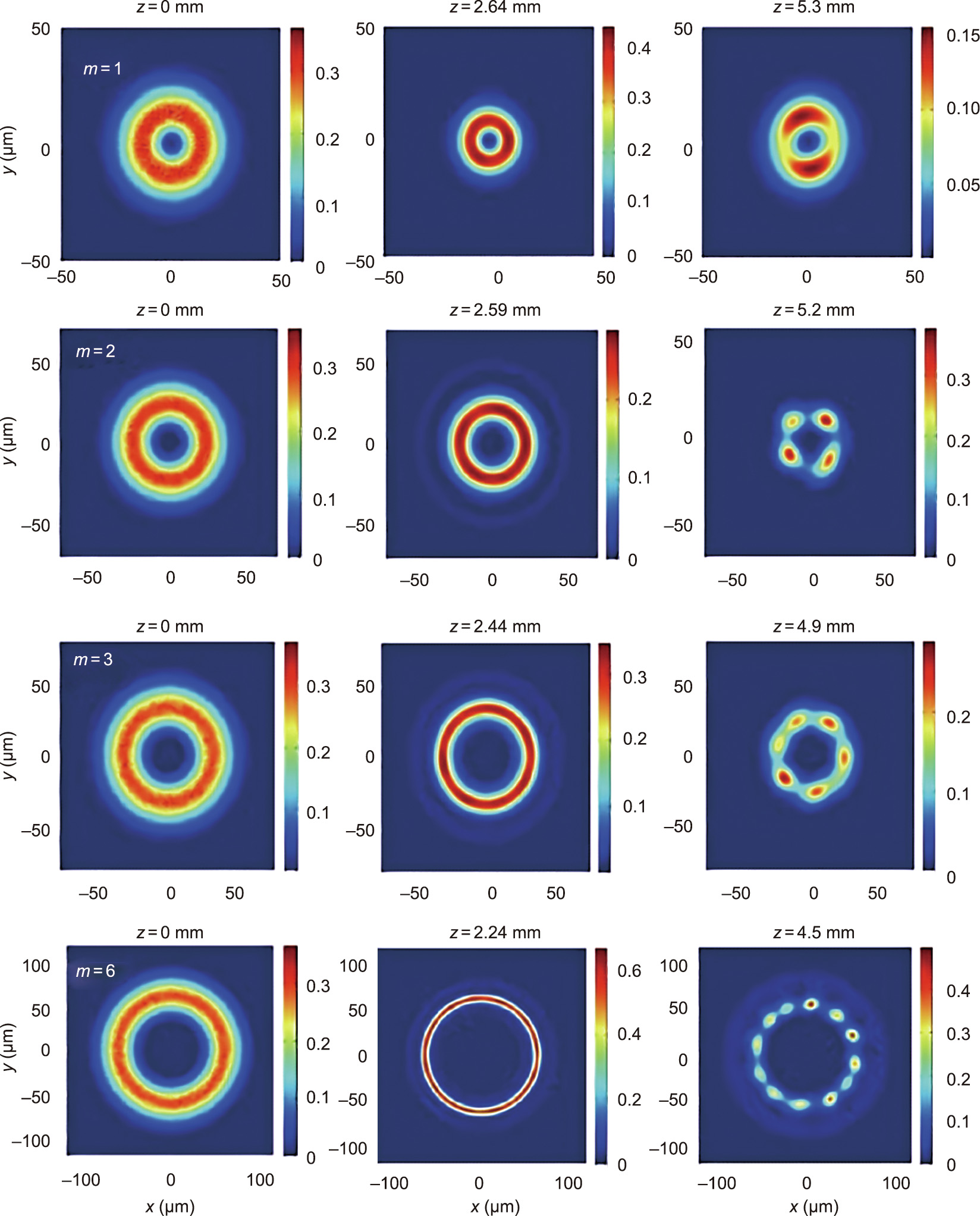
Fig. 10. Intensity distribution displaying the NB formation for initial topological charges m = 1, 2, 3, and 6 in a negative polarizability suspension. Reproduced from Ref. [49] with permission.
《Fig. 11》
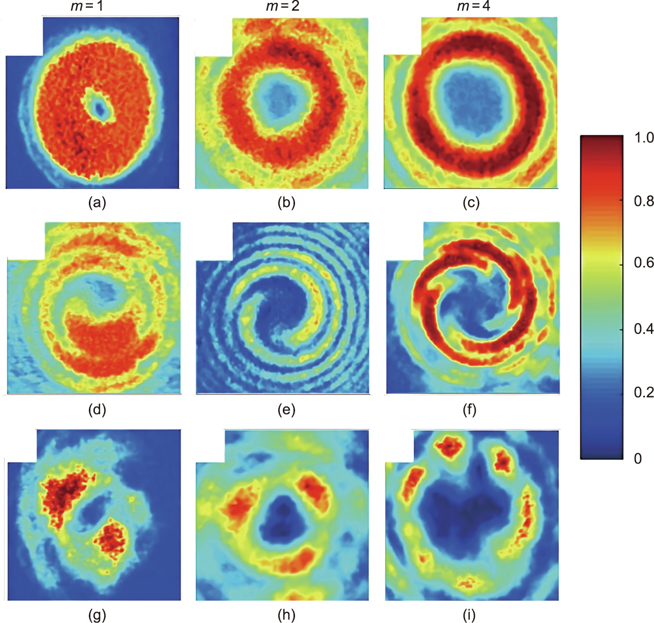
Fig. 11. Experimental evaluation displaying the generation of NBs in a negative polarizability suspension. (a–c) Intensities of the initial vortices with topological charges (a) m = 1, (b) m = 2, and (c) m = 4. (d–f) Interferograms for each initial optical vortex in (a–c), respectively. (g–i) NBs intensities after propagation for the input beams in (a–c), respectively. Reproduced from Ref. [51] with permission.
《4.2. Modulational instabilities in EVs》
4.2. Modulational instabilities in EVs
Depending on the initial beam, deriving expressions for both and can be quite challenging. Here, we consider two different classes of asymmetrical beams: EVs and HOBBITs. For the latter, we perform computational calculations to obtain values for and and estimate the number of modulations after its breakup through the MI gain. After solving the equations for  we obtain
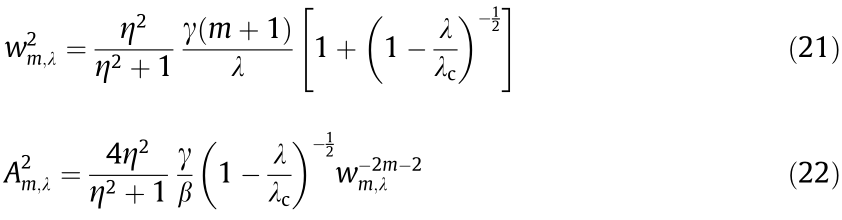
where  and
and  with
with  In the above expressions, the term
  = 1 +
= 1 +  appears due to the elliptical symmetry of the problem, with
The beam breakup into filaments due to the azimuthal MI can be studied by means of a perturbative method [48]. We consider perturbations along the mean radius  and the amplitude of the steady-state solution
  Here, the perturbed solution can be written as

where the variables in the above expression are the same as in the circular optical vortex case, except for the perturbed amplitude 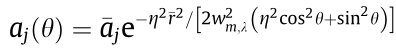
 with j=1, 2. The eigenvalue problem for EVs reads
where
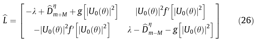
with  the prime denotes the derivative with respect to the argument, and
In the above expression, the parameter  = 0, M, –M is associated with all three possible values of the perturbed azimuthal charges indices in Eq. (24). By solving the system described above, one can obtain an expression for the propagation constant
 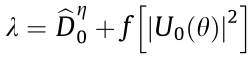 and another for the MI gain,
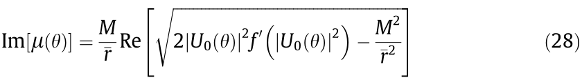
For a regular circular vortex, the approximate number of modulations along the azimuthal angle is given by the value or M where Im[μ(θ)] is maximum. Additionally, one can determine the distance where M modulations is observed is inversely proportional to the MI gain value at this point. However, for EVs, the beam is not azimuthally symmetric and the MI gain depends on the azimuthal angle. This means that a new approach should be used to get those insights.
An average of the MI gain maximal values over the azimuthal angle Gloc(θ), using as weights the value of M corresponding to the maximal MI gain at that angle nloc(θ), can be used to obtain the expected number of modulations along the EV:
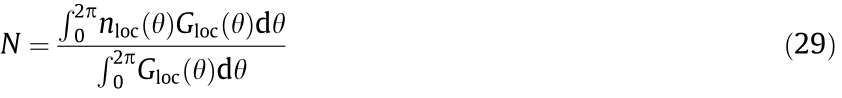
Fig. 12 presents the MI gain curves as a function of the perturbed azimuthal index M and the azimuthal angle θ for the topological charges m = 2 and m = 8, varying different values of η. We observe that, for small values of m, the vortex becomes more unstable as η decreases. In addition, the number of modulations N remains approximately the same for this case. On the other hand, as we increase m, N increases when η decreases.
《Fig. 12》
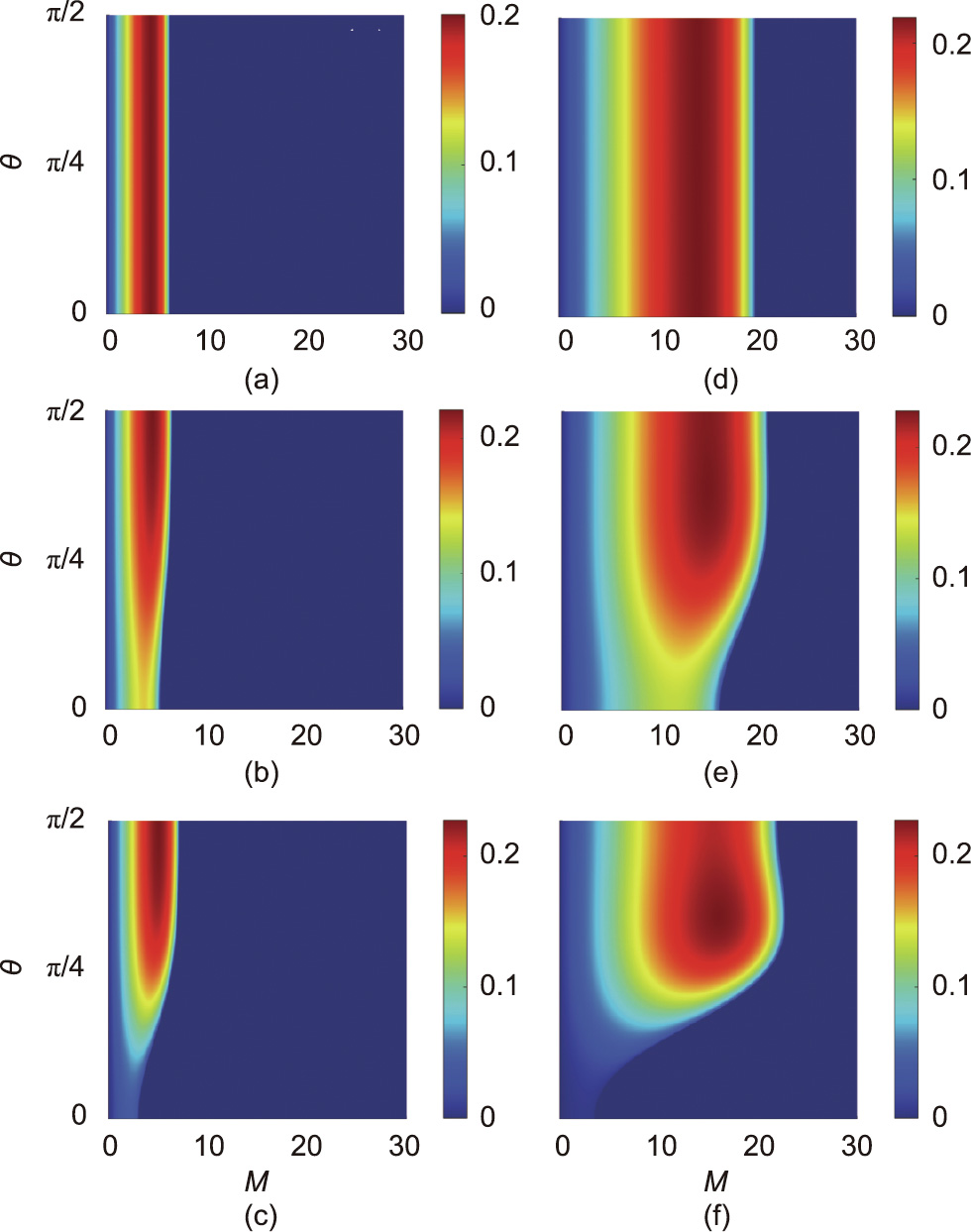
Fig. 12. Modulational instability gain Im[μ(θ)] curves as a function of the perturbation azimuthal index M and the azimuthal angle θ for various values of elliptical parameter η and topological charges (a–c) m = 2 and (d–f) m = 8. The values for η are indicated in each respective curve.
To validate the analytical predictions, a numerical simulation is performed by solving Eq. (12) using a beam propagation method [65,66]. As the input beam, Eq. (3) with the wavelength  = 532 nm was considered and, 10% random noise was added to quicken the growth of the MI. Here, we considered a negativepolarized nanocolloidal suspension (np < nb) consisting of air bubbles with a radius of 50 nm and a refractive index of np = 1 that is evenly distributed in water (nb = 1.33), with the filling factor
  The dynamics of the vortex propagation for different ellipticity parameters η are displayed in Figs. 13 and 14 for the topological charges m = 2 and m = 8, respectively. The first column indicates the initial steady-state solution with the noise, while the second column corresponds to the NB due to the azimuthal MI. The input power levels
  used are the values in which the beam width remains constant along the propagation. For higher (lower) power levels, the self-focusing effect (diffraction) starts to dominate the dynamics. The number of modulations remains unchanged for different values of η for low-order topological charges and becomes less stable as the beam gets more elliptical. The higher the topological charge m, the higher the number of modulations when η assumes smaller values. Additionally, the rotation along the propagation is also observed here as previously reported [34].
《Fig. 13》

Fig. 13. Intensity distributions of |U|2 (1013 V2 ∙m–2 ) for an EV with a topological charge m = 2, where each elliptical parameter and power levels are (a) η = 1.0 (P1.02 = 6.6 W), (b) η = 0.8 (P0.82 = 7.5 W), and (c) η = 0.6 (P0.62 = 11 W).
《Fig. 14》
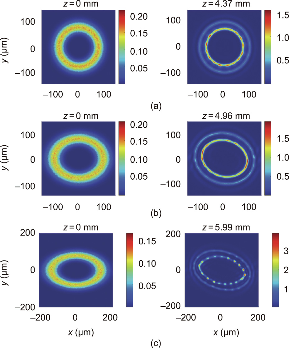
Fig. 14. Intensity distributions of |U|2 (1013 V2 ∙m–2) for an EV with a topological charge m = 8, where each elliptical parameter and power levels are (a) η = 1.0 (P1.08 = 46 W), (b) η = 0.8 (P0.88 = 52 W), and (c) η = 0.6 (P0.68 = 56 W).
Notice that, as we propagate the input beam, MI first acts around θ = π/2 and θ = 3π/2, rather than around other points. This can be explained by making a geometrical analysis of the elliptical beam interacting with the nanocolloidal suspensions. The radius associated with the local curvature at θ = π/2 is bigger than that at θ = π. Thus, the power needed to stabilize a circularly symmetric vortex at θ = π/2 is higher than what is needed for the smaller radius at θ = π. Because of this, the MI takes more time to act at θ = 0, π than at θ = π/2, 3π/2. Naturally, the beam stability along the propagation is also affected by the symmetry dependence of the power distribution. As the topological charge increases, the radius associated with the local curvature along the beam profile changes more slowly, leading to a more constant distribution of power around the semi-minor axis of the ellipse. In opposition, the curvature along the field distribution of low-order EVs changes more rapidly, and the power distribution is more uneven. This discrepancy in the power distribution strongly affects the longitudinal and transverse position where the MI takes place, leading to a more (less) stable propagation of EVs with higher (lower) topological charges. Fig. 15 provides a better visualization.
《Fig. 15》
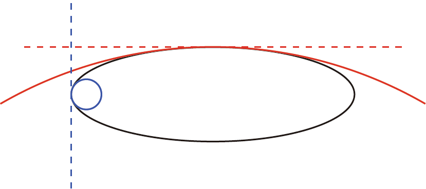
Fig. 15. Schematic figure for a better visualization of the MI action at different points of the ellipse. At θ = π (blue lines), the circle with a radius equal to the inverse of the local curvature is smaller than the circle at θ = π/2 (red lines). The tangent lines at both positions are denoted by dashed lines.
《4.3. HOBBIT beams》
4.3. HOBBIT beams
As introduced in the previous section, we must solve the equations for  retrieve the values for the beam width and amplitude = 0. The first step is to construct a surface for the action
  with respect to the beam width and amplitude, and then calculate the intersections between
 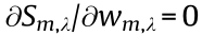 and
and 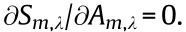 The point where the two curves intersect corresponds to the values of , that solve the variational problem
  = 0. Fig. 16 shows the action surface and the intersection curves for the topological charges m = 1 and 2, respectively.
The field distribution for the HOBBITs is strongly asymmetric with respect to the azimuthal angle θ, which means that the MI gain in Eq. (28) also depends on θ, and the expected number of modulations can be calculated using Eq. (29). Fig. 16 shows the MI gain surfaces as a function of the perturbation azimuthal index M and the azimuthal angle θ for the topological charges m = 1 and 2. The overall behavior in this case is similar to regular ring-shaped vortex beams previously reported, but the distance for the beam breakup due to the MI decreases as m increases. However, HOBBITs appear to be more stable upon propagation in colloidal media, when compared with both regular beams and EVs, since the modulations take place at a longer distance when compared with the other beams.
《Fig. 16》
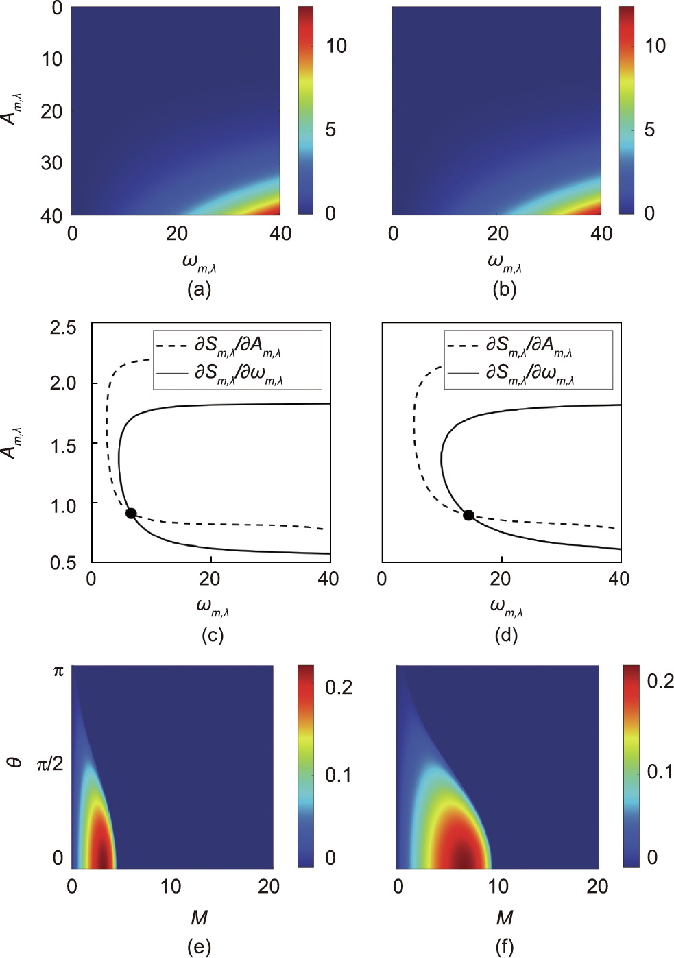
Fig. 16. Numerical method to construct the MI gain surfaces. Action surface for (a) m = 1 and (b) m = 2. Intersection between the curves for  = 0 and
  = 0 with (c) m = 1 and (d) m = 2. Im[μ(θ)] curves as a function of the perturbation azimuthal index M and the azimuthal angle θ for (e) m = 1 and (f) m = 2.
Following the same procedure presented before, we performed numerical simulations solving Eq. (12) using the same parameters considered in the previous section. Here, the beam parameters used were ρ0 = 8.6 μm and β = 0.6. Fig. 17 shows the evolution of HOBBITs in nanocolloidal media with negative polarizability for the topological charges m = 1 and 2. Following the numerical procedure presented in this section, one can predict the number of modulations for asymmetrical beams too. For this case, the expected number of modulations matches the results observed after simulating such dynamics through Eq. (12). Similarly to the case of the EVs, as we increase the HOBBIT’s topological charge, the breakup distance also increases. Additionally, we highlight that the beam rotation is again observed upon propagation. This is expected for propagating non-circular beams, as reported in Refs. [34,67]. One can directly calculate this rotation by performing a Fourier transform of the input beam for free-space propagation, and the same is observed under interaction with the considered saturable media.
《Fig. 17》
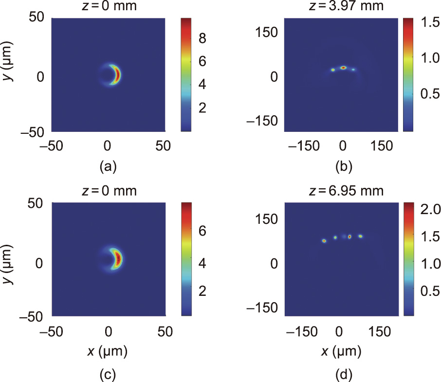
Fig. 17. Intensity distributions of |U|2 (1013 V2 ∙m–2) for a HOBBIT with the topological charges and power levels (a, b) m =1 (P1 = 13 W) and (c, d) m = 2 (P2 = 15 W).
《5. Conclusions》
5. Conclusions
In this article, we reviewed complex-shaped OAM beam propagation in nanocolloidal media with saturable nonlinearity. In the first part, an overview of the nonlinear response of circular optical vortices propagating through nanosuspensions was presented. Non-cylindrical optical beams were also considered, followed by an analytical approach for EVs and numerical calculations for HOBBITs. We find that, in the case of the beams lacking cylindrical symmetry, the MI gain surface depends on the azimuthal coordinate θ and requires a revised procedure to predict the NB formation based on the averaged MI gain. This revised approach was shown to be in good agreement with the results of full numerical simulations for moderate values of topological charge. However, as the topological charge was increased above a certain value (e.g., m > 10), the analytical predictions deviated from those obtained in the numerical simulations. These deviations are, in fact, expected even in the case of cylindrically symmetric vortices, since the flat region associated with the maximum values of the MI gain surface becomes larger and, as a result, several values of M for the perturbations experience approximately the same MI gain and thus have equal probability to grow. This conclusion suggests that a new approach must be developed to predict NB formation in colloidal media for higher-order vortices. A realistic optical communication protocol using OAM as orthogonal states, propagating in either air or water, it will possibly encounter particles suspended due to the non-static nature of the medium [68]. Additionally, one can make use of the refractive index different between the particles and the background to develop new methods of optical channel cleansing. Concerning other applications, understanding how light interacts with particle suspensions might be useful to develop or improve imaging systems [69], sensing techniques [70], and optical tomography [71], to cite a few. Within compact systems, one can make use of metasurfaces to generate optical beams carrying OAM in micro- or nanoscale. For instance, the usage of metasurfaces both increase transmission efficiency and facilitate the generation of optical vortices in sufficient small systems such as chemical aqueous environments and biological suspensions.
《Acknowledgment》
Acknowledgment
We acknowledge the support from the Office of Naval Research MURI (N00014-20-1-2550).
《Compliance with ethics guidelines》
Compliance with ethics guidelines
D. G. Pires and N. M. Litchinitser declare that they have no conflict of interest or financial conflicts to disclose.


 京公网安备 11010502051620号


