《1. Introduction》

1. Introduction

In recent years, the use of biomimetic robots has successfully promoted the understanding of a wide range of animal behaviors [1,2]. Using effective control methods and active guidance, biomimetic robots can interact with animals to observe and record their responses [3–7]. Sometimes, biomimetic robots are placed in a group of animals to explore their behavior patterns or verify scientific hypotheses in the process of interaction [8–11]. For biomimetic robots, lifelike behaviors can improve the effectiveness of their interactions with animals. For example, when robots simulate body movements related to foraging behavior, finches will spend more time on foraging [12]. The tail swinging behavior of a robotic fish will have a substantial impact on the movement of fish [3]. Moreover, biomimetic robots with similar behaviors can greatly improve the modeling of complex animal behaviors [13,14].

The social activities of rats have aroused the interest of many researchers, and these studies have led to remarkable achievements [15,16]. Because of the advantages of biomimetic robots in animal interaction, various kinds of robots have been designed for the behavioral study of rats [17–21]. However, these robots have fewer degrees of freedom (DOFs) and lack flexibility in local movements, which makes it difficult to realize a natural interaction process. In our latest work, we simplified the DOFs of rats, extracted four DOFs in the pitch direction and three DOFs in the yaw direction, and used them to design the bionic spine mechanism of a robotic rat [22]. Although the robot can perform some basic rat-like movement primitives (MPs) with high flexibility, it is difficult for them to simulate the behavior characteristics of rats. Moreover, it is difficult for the robot to adapt to a variety of rat movement parameters and it does not have the ability to generalize movement. Therefore, we hope to both build a behavior model for rats and learn and generalize the spinal joint trajectory to control the robot so that it produces rat-like behaviors.

Many modeling methods for animal behaviors have been proposed. Ding et al. [23] used a central pattern generator (CPG)- based method to model the behavior of amphibians and realize a multi-modal behavior design. Ren et al. [24] used a general internal model (GIM)-based biomimetic learning method to model the behavior of fish and achieved similar swimming patterns on a multi-joint robotic fish. These modeling methods are suitable for animals with rhythmic movement, whereas the movements of rats, especially the trajectory of spinal joints, are diverse and not rhythmic; hence, the above modeling methods are unsuitable. Leos-Barajas et al. [25] used hidden Markov models (HMMs) with hierarchical structures to model the behaviors of harbor porpoises and garter snakes. Cullen et al. [26] used non-parametric Bayesian methods to estimate the behavior of rostrhamus sociabilis more accurately than an HMM. HMM and Bayesian methods are based on probability distributions and transitions, which are more suitable for the analysis of rat behavior. However, the observed data in an open-field test revealed that the movement of rats is usually generated by a combination of MPs. It is challenging to deal with the combination and timing of these MPs using the abovementioned modeling methods. If the probability statistics of MPs are analyzed directly, it is difficult to capture the behavior characteristics of rats and will disrupt the inherent combinations of MPs.

To better reflect the behavior characteristics of rats, we first combined the MPs in a time sequence, and the features of these combinations are reflected by a set of attributes. Each combination represents a rat movement. Using these attributes, we associated different combinations with different behaviors using the softmax classifier to learn the relationship between them. Using the classification results, we established the behavior–movement hierarchical probability model. In the hierarchical model, we not only represent the corresponding relationship between behaviors and movements and the transitions between different behaviors, but also the introduced states. This is because we hope to use states to further distinguish different behaviors and deepen our understanding of animal behaviors. Moreover, these different states may reflect different emotions in rats, which is an important consideration in future interaction experiments. The convergence and control of the model ensures its accuracy.

In addition to behavior modeling, we need to learn the rules of rat movements. The MPs of rats can be described by static and dynamic parameters. The static parameters determine the movement amplitudes, average speeds, frequencies, or durations, whereas the dynamic parameters determine the angle and angular velocity of each spinal joint with respect to time. The MPs of rats usually consist of a variety of static parameters. Even for the same set of static parameters, different dynamic parameters may be present. To reduce computational complexity, we carried out cluster analysis on these parameters. We used hierarchical clustering and fuzzy Cmeans (FCM) clustering to extract the predominant values of the static and dynamic parameters, respectively [27,28]. The predominant parameters were then used to fit the spinal joint trajectory of rats. Obviously, the fitting accuracy of joint trajectory depends on the results of cluster analysis. However, each clustering method has its own shortcomings. Hierarchical clustering does not need a predetermined number of clusters, but once a merge has been executed, it cannot be modified, and the quality of clustering is limited; the FCM clustering needs a predetermined number of clusters, and it often falls into locally optimal solutions [29,30].

Additionally, we hope that learning rat movements will not remain at the level of copying, but lead to the ability to generalize. That is, we can infer a rat’s spinal joint trajectory for certain movement parameters through the supervised learning of the test samples. To improve the accuracy of movement generalization, we need a variety of movement parameters as the input of a neural network. This runs counter to our aim to reduce computation. To solve the uncertainty in clustering quality and balance the amount of computation with generalization accuracy, we used the Pearson correlation coefficient to measure the similarity between the robotic rat and rats. The results of clustering were modified to control the extraction of movement parameters.

Although we have developed a similar quadruped robotic rat, it moves slowly and finds it difficult to achieve a high body pitch angle, which is not conducive to interaction with actual rats. Therefore, the hind limb of the robotic rat was transformed into a base that includes a hip servo motor and four wheels (two front driving wheels and two rear universalwheels).When the ratmoves in a straight line, the angular speed of the driving wheel is determined by the average forward speed and radius of the wheel.When the rat turns, because the driving wheel only rotates around the axis and lacks a DOF for lateral movement, this will inevitably cause differences between the robotic rat and actual rats. To maximize the similarity of the robotic rat when turning, we used the learned rat spinal joint trajectory to drive the yaw joints of the robotic rat and control the difference in the rotation speed of the two driving wheels to generate the turning movement.

The main contributions of this paper are as follows:

(1) We regarded a rat movement as a temporal combination of MPs and defined the attributes of these combinations. Rat behavior is classified by different combinations of attributes. The hierarchical probability model better reflects the behavior characteristics of rats. This lays a foundation for future robot–rat interactions.

(2) By training a neural network, we can predict the trajectory of each joint of the robot using only a set of static parameters, which greatly simplifies the movement planning process and facilitates the real-time planning of the robot.

(3) We controlled the extraction process of the rat movement parameters by modifying the results of cluster analysis. This allows us to reduce the amount of calculation and ensure a high similarity between the robot and rats.

《2. Material and methods》

2. Material and methods

Our approach is summarized in Fig. 1. In the process of behavior modeling, we first obtained the time series of MPs by tracking the coordinates of marked points. Then, we formed the movement of rats using MPs and combination attributes. A softmax classifier was used to classify the behaviors and states of the rats. Through the sequence of MPs and the results of classification, we established a hierarchical model of rat state, behavior, and movement in a probabilistic way.

《Fig. 1》

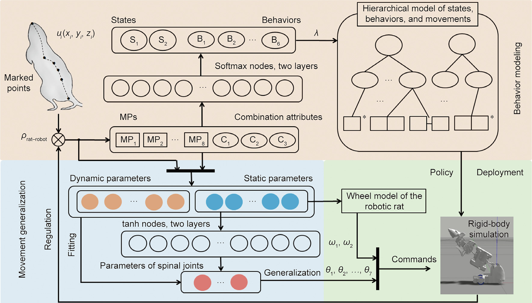
Fig. 1. Generation process of rat-like behavior for the robotic rat. In the process of behavior modeling (light red box), we proposed a classification method for rat behaviors (B₁, B₂, ..., B₆) and states (S₁ and S₂), and obtained the hierarchical model of the states, behaviors, and movements. In the process of movement generalization (light blue box), we extracted the movement parameters of the rats and realized the mapping from static movement parameters to joint trajectory parameters. In the deployment on the robot (light green box), we controlled the robot by the policy and commands. The hierarchical model was used as the policy, and the generalized spinal joint angular displacement (θ₁, θ₂, ..., θ₇) and wheel angular velocity (ω₁, ω₂) were used as the commands for the simulation model. The correlation coefficient between the robotic rat and rats (ρ_rat–robot) was used to measure the similarity and to regulate the process of behavior classification and movement parameter extraction. u_i(x_i, y_i, z_i): coordinates of the movement joints; : initial and transition probabilities between different states and behaviors as well as the observation probability of each combination in each kind of behavior; C₁, C₂, and C₃: combination attributes of MPs; tanh: hyperbolic tangent. 

In the process of movement generalization, we extracted the static and dynamic movement parameters of each combination of MPs. These parameters were used to fit the trajectory parameters of the rat spinal joints (in the form of a Fourier series). To realize the generalization of movement, we established the mapping relationship between the static movement parameters and joint parameters using a back propagation (BP) neural network.

In the deployment on the robot, we deduced the relationship between the static movement parameters and angular velocity of the driving wheel using the wheel model of the robot. The hierarchical model was provided to the robot as a control policy, so that the robot understood what kind of behavior and movement should be planned in a more natural and biomimetic way. Through the movement planning, we identified the probability distribution of the static movement parameters under each movement and obtained the trajectory of each joint, so that the robot can perform these behaviors and movements. The correlation coefficient was used to measure the similarity between the robot and rats and control the process of behavior classification and extraction of movement parameters in an iterative manner. In the following text, we describe each component in detail.

《2.1. Behavior modeling》

2.1. Behavior modeling

2.1.1. MPs, behaviors, and states of rats

An open-field test is used to study the spontaneous activity of animals in a new environment. It allows experimental animals to move freely in a certain space with few restrictions and has become an important method for studying the behavior and movement of animals [31,32]. Biologists usually divide the MPs of rats into motions such as going straight, turning, standing up, and staying in one place. Correspondingly, the behaviors of rats are divided into behaviors such as exploring, grooming, and resting to reflect the different activity characteristics of rats [33,34]. In this paper, we observed the activities of individual rats (Rattus norvegicus) in a1m × 1 m × 1 m open field, recorded 10 min daily, and obtained a dataset of the motions of three rats over five days. The rats involved in this study were from the same litter and were seven weeks old. The dataset (150 min) contains 3537 rat movements. 

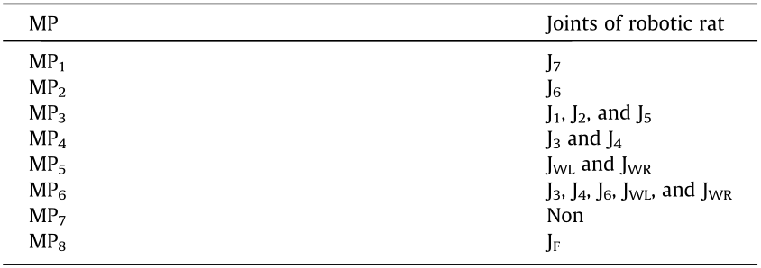
Here, we marked the nose tip, tail, and key movement joints of the rats, and tracked the coordinates of these points through multiple cameras. We defined the MPs based on the coordinate changes of the marked points. The pitch and yaw of the head joint are defined as MP₁ and MP₂, respectively; the pitch and yaw of body joints are defined as MP₃ and MP₄, respectively; the linear motion of all marked points is defined as MP₅; the rotational motion of all marked points is defined as MP₆; almost no motion in the coordinates of all marked points is defined as MP₇; and the swing of the forelimb joint is defined as MP₈. The MPs, behaviors, and states of the rats are presented in Table 1.

《Table 1》

Table 1 MPs, behaviors, and states of rats.

2.1.2. Combinations of MPs and classification of behaviors and states

An observed sequence of MPs is shown in Fig. 2. The sequence of MPs reflects the activity sequence of the rats, and the movements of the rats can be represented by a temporal combination of the above MPs. We extracted the combinations of MPs using the following method: First, we calculate the distance between MPs. A value of 0 indicates that the MPs occur simultaneously. We further extract all MPs that occur simultaneously and form candidate combinations (including the combination that contains only one MP). Secondly, each combination is combined with the subsequent MP or combination (with a distance value of 1) to form a new combination and the frequency of the new combination is calculated. If the frequency of the new combination is very high, the new combination replaces the original combination; if the frequency of the new combination is high, both combinations are retained; if the frequency of the new combination is low, the new combination is discarded. The second step is repeated until no new combination appears.

We use combination attributes to reflect the features of the combinations of these MPs. Here, C₁ represents the repeatability of MPs, where 1 represents repetition and 0 represents non-repetition; C₂ represents the number of MPs generated simultaneously; and C₃ represents the number of MPs in the combination (juxtaposed MPs count as only one). Then, we classified the behaviors and states on the basis of different combinations of MPs (Fig. 2). 

《Fig. 2》

Fig. 2. Observed MP sequence. C₁, C₂, and C₃ correspond to different behaviors and states.

We used supervised learning to obtain the relationship between the combination of MPs and behaviors/states. A labeled dataset was collected to train the softmax classifier. The inputs of the network are MPs (1 indicates that the MPs are activated, whereas 0 indicates that they are not activated) and combination attributes, and the outputs are the corresponding behaviors and states. The number of nodes in the hidden layer is eight. Here, we assumed that different behaviors and states are mutually exclusive, which is conducive to robotic rat control.

2.1.3. Hierarchical model of states, behaviors, and movements

The results of the softmax classifier were used to obtain the hierarchical model of states, behaviors, and movements (Section 3.1). Here, denotes the initial and transition probabilities between different states and behaviors as well as the observation probability of each combination in each kind of behavior. This hierarchical model effectively reflects the activity characteristics of the rats in the observation. The state layer of the structure is a Markov model and includes an initial probability, a probability for transition to its own state, and a probability for transition to other states; for the behavior layer, because a continuous behavior is represented by a specific combination of MPs, it only has an initial probability and a probability for transition to other behaviors; for the movement layer, because there is not necessarily a connection between the combinations of MPs corresponding to different behaviors, which is extremely random and dominated by the probability of transition between different behaviors, only an the initial probability (the observation probability) is given. The hierarchical model becomes gradually more refined from top to bottom as the probability system becomes simpler. In the following work, we analyze the convergence of the model. We also adjust the model using the correlation between the robot and rats.

2.1.4. Model convergence

Information entropy solves the problem of the quantitative measurement of information [35]. In this study, we calculated the information entropy of the states and behaviors in the hierarchical model to determine whether the model tends to be stable with respect to probability. We first counted 1700 rat movements, mapped these movements to different states and behaviors, and then calculated the number of occurrences and probability of each state and behavior. Next, the probability distribution of each state and behavior was recalculated for each additional 200 rat movements. When the probability distribution of each state and behavior hardly changed, the information entropy of the states (H(S)) and behaviors (H(B)) also become stable, indicating that the model had converged. The calculation of information entropy is as follows:

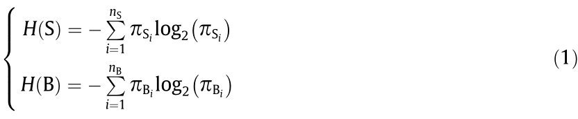
where n_S and n_B represent the number of states and behaviors in the model, respectively; and are probability of each state and behavior in the model, respectively.

The calculation results are shown in Fig. 3. The information entropy of states and behaviors in the model is stable at around 3500 rat movements. The increase in information entropy indicates that the difference in probability between different states and behaviors is decreasing. This may reflect the adaptability of rats to a new environment. In the early data, the probabilities of stressed states and exploratory behavior are much higher than the other states; as the amount of data increases, the probability of relaxed states, resting, grooming, and other rat behaviors gradually increased. After the model converged, we stopped collecting data from the rats.

《Fig. 3》

Fig. 3. Information entropy of states and behaviors.

2.1.5. Model regulation

The Pearson correlation coefficient reflects the linear correlation between two sets of data, and it has been successfully used to measure the movement similarity between biomimetic robots and animals [36,37]. Here, for a particular combination of MPs, we used u_i,rat to represent the coordinates of the movement joints of rats, and u_i,robot to represent the coordinates of the movement joints of the robotic rat. The movement correlation coefficient () between the robotic rat and rats can be expressed as follows: 

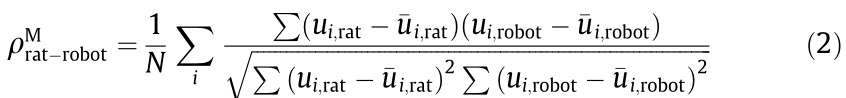
where N represents the number of movement joints. Furthermore, for a certain kind of behavior, assuming that it includes K different combinations and the observation probability of each combination is  the behavior correlation coefficient () between the robotic rat and rats can be formulated as follows: 

To achieve rat-like behavior in the robotic rat, we required that the behavior correlation coefficients be greater than 0.8. When the correlation coefficient of a certain kind of behavior is below this threshold, we first adjust the extraction process of the movement parameters (Section 2.2); if it still fails to meet the threshold, the combinations to which the behavior belongs are split so that they corresponding to different new behaviors, and then the behaviors are reclassified. A realistic example is described in Section 4.

《2.2. Movement generalization》

2.2. Movement generalization

Our parametric modeling of rats is shown in Fig. 4. The red markers indicate the main DOFs in the pitch direction, the blue markers indicate the main DOFs in the yaw direction, and the black markers indicate the nose tip, tail end, and center of mass (CoM) of the rats. A coordinate system was set up with respect to the tail of the rats, and the Kinovea software was used to track the location information of the marked points.

《Fig. 4》

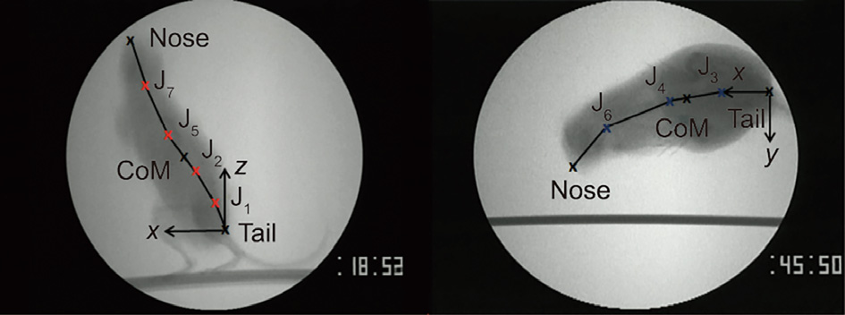
Fig. 4. Parametric modeling of rats. The red markers (J₁, J₂, J₅, and J₇) and blue markers (J₃, J₄, and J₆) indicate the main DOFs in the pitch and yaw directions of the rats, respectively, and the black markers are used as the reference points to define the static movement parameters.

We define the static movement parameters, and all angles refer to the movement amplitudes of rats. The pitch angle is zero in the horizontal position, positive upward, and negative downward. The yaw angle is zero at the symmetrical position (where the angles of the rat head and body are in a straight line), the direction is random, and the value is positive (it was observed in the data that the probabilities of rat left and right yaw are roughly equal). Parameters head pitch angle φ_hp and head yaw angle φ_hy represent the angle between the x-axis and the line from the nose tip to joints J₇ and J₆, respectively. Parameters body pitch angle φ_bp and body yaw angle φ_by represent the angle between the x-axis and the line from the CoM to the tail end. Parameter turing angle α represent the rotation angle of the x-axis before and after the turning movement. Parameter φ_fs represents the rat forelimb swing angle, v represents the average forward speed of the rat CoM, represents the movement frequency (only for combinations with repetitive MPs), and T represents the movement duration.

To extract the predominant values of the static parameters, because of the small sample size and the difficulty in determining the number of clusters in advance, we used hierarchical clustering to classify these static parameters. First, we treated the different values of each static parameter as a class, and calculated the distances between classes. The two closest classes (i –1, j –1) were merged into one, and the average value of the original two classes was taken as the value of the new class. Afterwards, the distances D_i,j between the new class (j) and other classes (i) were calculated, until the distance between the two classes met the following condition:

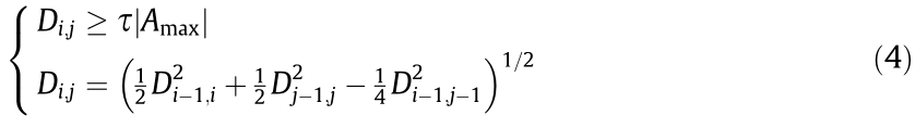
where A_max denotes the maximum value of each static parameter and τ determines the density of classification. Finally, the static parameter value corresponding to each class in the clustering results is the extracted dominant value. When the probability corresponding to the predominant values of a static parameter is calculated, it is often affected by other parameters. Therefore, it is necessary to calculate the independence between the two parameters and determine the joint statistics of two non-independent parameters to form the joint probability distribution of the predominant values; otherwise, separate statistics for each parameter are obtained to form the independent probability distributions of the predominant values.

To extract the predominant values of the dynamic parameters, because of the large amount of data and accurate classification requirements, we used FCM clustering to classify the dynamic parameters. In this paper, the dynamic parameters (θ_i,j) mainly reflect the position characteristics of the main DOFs over time. For a joint in a certain kind of movement, we can calculate its angular displacement and angular velocity at a discrete time by the marked coordinate values. Because this kind of movement occurs many times, we obtained the data group 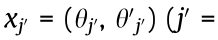 1, 2, ..., n) of the joint under a specific set of static parameters. Here, 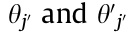are the angular displacement and velocity of joint J_i at time t_j, respectively. The process of cluster analysis is expressed as follows: 

where 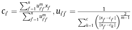 and O denotes the objective function, denotes the membership degree of sample  belonging to class , m is the factor of membership degree, which affects the degree of classification, and denotes the clustering center of class . The number of clusters c is determined by the average value of the contour coefficient of each sample point. When the average value of the contour coefficient is closer to 1, this indicates the clustering is better. Parameters and iterate continuously, until the objective function O is less than a certain threshold. To better reflect the movement characteristics of rats, we used the weighted method for each sample instead of the average method for the predominant dynamic parameters. The weight of each sample was determined by the proportion of the number of samples of each class as follows:

where parameter denotes the set of all samples of class and denotes the number of samples contained in class .

Because functions satisfying Dirichlet’s condition can be approximately expressed by a finite Fourier series, we used a Fourier series to simulate the angular displacement curve of each joint in rats [38]. After experiments, we found that a second-order Fourier series is sufficiently accurate (R-square > 0.9). Taking the pitching movement (MP₁MP₃) under exploring behavior (B₂) as an example, the input and output are normalized and the following formula is obtained:

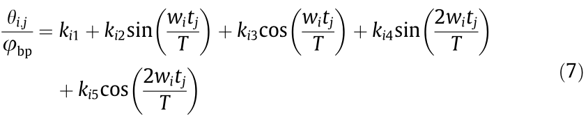
where, w_i and k_i1–k_i5 are fitted joint trajectory parameters (i = 1, 2, 5, and 7). For a repetitive movement such as MP^*₁, w_i are represented by frequency . 

A neural network is usually used to generalize joint movements [39–41]. In this study, we adopted the BP neural network with two hidden layers. The inputs of the network are static parameters, and the outputs are joint trajectory parameters. The hyperbolic tangent (tanh) activation function is used to accelerate the convergence of the network. According to previous studies [42,43], the number of nodes in the hidden layer should be between the number of input nodes and output nodes, and the same number of neurons is used for all hidden layers. In this study, for each combination of MPs, a corresponding neural network was used to participate in the training process. We adjusted the number of nodes in the hidden layer to avoid the phenomena of underfitting or overfitting. Still taking the pitching movement (MP₁MP₃) under exploring behavior (B₂) as an example, the number of input nodes of the network was two (φ_bp, T), the number of output nodes was six (w_i , k_i1–k_i5), and the number of nodes in the hidden layer was four (as shown in Fig. 5). The cost function was the mean squared error loss function and the network was trained by a batch sample parallel gradient algorithm. The clustering results were modified to adjust the static and dynamic parameters. In the initial setting, to reduce the complexity and computation of the model, we used a larger value τ and a smaller value c. When the correlation coefficient of a certain kind of behavior is below a threshold, the clustering results of movements are modified in descending order of observation probability while reducing the τ value and increasing the c value. 

《Fig. 5》

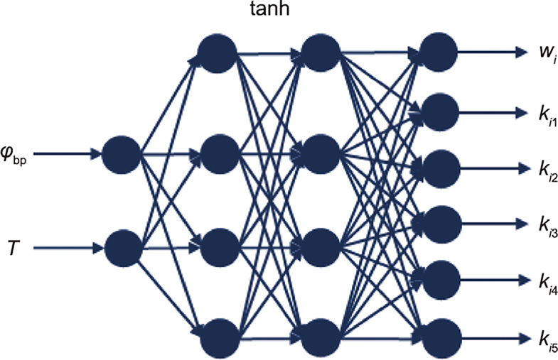
Fig. 5. BP neural network used in the pitching movement (MP₁MP₃) under exploring behavior (B₂).

《2.3. Deployment on the robotic rat》

2.3. Deployment on the robotic rat

2.3.1. Robotic rat platform

The prototype of our recently developed robotic rat is shown in Fig. 6(a). The robotic rat mainly consists of a head, forelimb, waist, and hip. The head and hip joints are driven by a servo motor, the waist joints and wheels are driven by a direct current (DC) motor, and the forelimb is driven by a micro deceleration stepper motor. Its shape and size are similar to those of actual rats, and the total mass is approximately 400 g. The spinal joints of the robot correspond to the main DOFs of the rats. Fig. 6(b) and Table 2 show the distribution of each joint of the robotic rat and the corresponding relationship between the MPs and joints.

《Fig. 6》

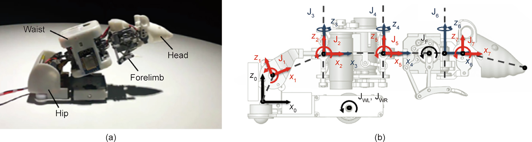
Fig. 6. (a) Robotic rat and (b) motion coordinate system of the robotic rat. J_F: forelimb swing joint; J_WL, J_WR: left and right drive wheel joint, respectively.

《Table 2》

Table 2 Joints of robotic rat used to perform the MPs.

The movement parameters of the robot are mainly affected by the movement parameters of rats and the structural constraints of the robot. The task space constraints on the MP mean that by analyzing the workspace of the robot and the interference between joints, we can obtain the amplitude of the movement parameters of the robot, such as the maximum body pitch angle and body yaw angle. We described this analysis in detail in Ref. [22]. Concerning the constraints on the control, the robot needs to maintain dynamic balance in movements without vibration or sideslip. Therefore, the robot usually has a minimum movement duration under various conditions. We analyzed this in detail in Ref. [44]. When determining the movement parameters of the robot, we depend on whether the extracted parameters of rats exceed the limits of the robot itself. If the limit is not exceeded, the movement parameters of the robot are equal to those of the rat; if the limit is exceeded, the movement parameters of the robot are equal to the maximum or minimum value of the limit. Hence, we defined the parameters of the robot movements as

where U and C_eq represent the task space and dynamic balance constraints, respectively; (φ_bp)_max and (φ_by)_max represent the maximum body pitch angle and body yaw angle satisfying the task space constraints, respectively; and T_min represents the minimum movement duration satisfying the dynamic balance constraints. Using the prototype, we built a rigid-body simulation model in the robot operating system (ROS) environment (Gazebo simulator) and used it in the training process.

2.3.2. Wheel model of the robotic rat

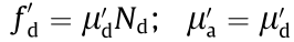The turning model of the robotic rat is shown in Fig. 7, where p is the instantaneous CoM of the robotic rat, q is its instantaneous rotation center, F_t and F_n are the tangential and normal static frictions, respectively. Parameters are the rolling friction on each wheel, which can respectively be expressed as  and  and  are the rolling friction coefficients. Parameters N_a, N_b, N_c,  and N_d are the support forces on each wheel, which can be expressed by the angular displacement θ_i of each yaw joint through the balance equations  for the robot turning model. Each link i is not only affected by moment of inertia, but also by the centrifugal and Coriolis forces in the noninertial frame. Force is the resultant force of the centrifugal force and Coriolis force applied to link i. Moreover, F_co is the composition of forces acting on all links, that is,  denotes the angle between F_co and x-axis. Parameter ω is the instantaneous turning angular velocity, R is the turning radius, and L is the track width. Based on Newton’s second law, for the turning movement of the robotic rat, the dynamic equations in the tangential and normal directions are written in Eq. (10): 

《Fig. 7》

Fig. 7. Turning model of the robotic rat. is the moment applied to link i.

The static friction and driving force of the wheels are the reaction forces, which are equal in value and not more than the sum of the maximum static friction on each wheel. The angular velocity of the CoM caused by the difference in rotation speed of the driving wheels is generated by the normal static friction. Based on the statistics of the static parameters of rats, the robotic rat must reach turning angle α within duration T. Assuming that the rotational speeds of the driving wheels a and d are ω₁ and ω₂, respectively; τ₁ and τ₂ are the actual output torques of the two driving wheels; and P₁ and P₂ are the actual output power of the two driving wheels. We then obtain the set of equations in Eq. (11):

where r_d is the radius of the driving wheel, k₁ and k₂ are power factors.

Because F_co and can be expressed by the angular displacement θ_i of each yaw joint, which depends on parameters α and T, the relationship between the driving wheel rotational speeds ω₁ and ω₂ and the parameters α and T can be obtained using Eqs. (10) and (11).

《3. Results》

3. Results

《3.1. Probability distribution and transition in hierarchical model》

3.1. Probability distribution and transition in hierarchical model

On the basis of behavior and state classification, we determined the probabilities of the states, behaviors, and movements by the number of occurrences, as shown in Fig. 8(a). Among them, the dotted lines represent the initial probability, the solid lines represent the transition probability, and different colors represent different probability intervals. For walking behavior, which includes going straight, turning, and staying MPs, because the behavior can include various combinations with different numbers of MPs, we created separate probability statistics. Fig. 8(b) shows the initial probability (black dotted line) and transition probability (black solid line) of each MP in walking behavior; Fig. 8(c) shows the probability distribution of the number of MPs in the combinations included in walking behavior.

《Fig. 8》

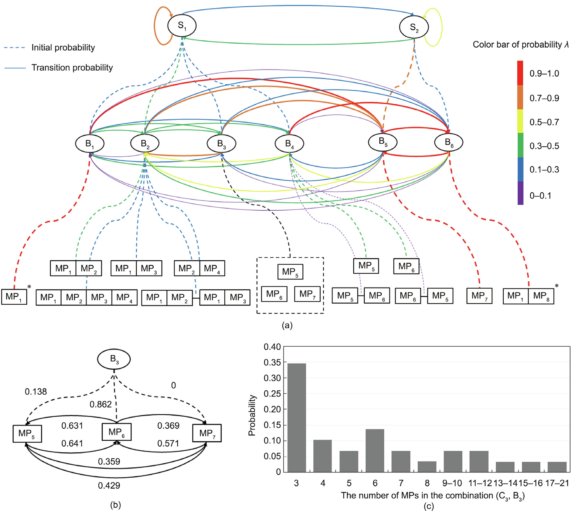
Fig. 8. Probability distributions and transitions in the hierarchical model. (a) The different colors correspond to different probability intervals, the juxtaposition of MPs indicates that these MPs are generated simultaneously, the symbol ‘‘–” indicates the time sequence of MPs and ‘‘*” indicates that the MPs occur repeatedly in the combination; (b) initial probability (black dotted line) and transition probability (black solid line) of each MP in walking behavior; (c) probability distribution of the number of MPs in the combinations included in walking behavior.

《3.2. Distribution of static parameters》

3.2. Distribution of static parameters

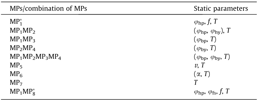
Table 3 shows the relevant static parameters used to describe the MPs and combinations of MPs. The parameters in brackets are not independent of each other. For different behaviors, the same MPs and static parameters often appear. Fig. 9 presents the distribution of the static parameters in different behaviors. Fig. 9(a) compares average forward speed during walking and trotting. In both cases, the average forward speed has a similar range (0.125–0.250 m·s^–1 ), but a high speed when trotting is more likely. Fig. 9(b) compares the staying times of walking and resting. The staying time in walking is short, approximately 0.5–1.5 s, whereas the staying time is longer in resting, approximately 3–7 s. Fig. 9(c) shows the distribution of the turning angle and movement duration in walking and trotting. The upper-right ‘‘*” indicates that the data has a high probability of occurrence (the sum of the occurrence probability of all data with ‘‘*” is greater than 0.7). It can be seen that the turning movement when trotting has a faster average angular velocity than that when walking. The distributions of these parameters support the rationality of the behavior classification.

《Table 3 》

Table 3 Static parameters used to describe the MPs/combination of MPs.

《Fig. 9》

Fig. 9. Distributions of the static parameters in different behaviors. (a) Comparison of average forward speed in walking and trotting; (b) comparison of the staying time in walking and resting; (c) distribution of the turning angle and movement duration in walking and trotting. The label ‘‘*” indicates that the data has a high probability of occurrence.

《3.3. Generalizable movement planning of the robotic rat》

3.3. Generalizable movement planning of the robotic rat

Fig. 10 presents the main joint trajectory curves of the pitching, yawing, and turning movements. The light red areas represent the envelope of the test sample trajectory, and the black solid lines represent the mean predicted value of the test sample trajectory given by the neural network based on the training samples. For each movement, the number of training samples is approximately twice that of the test samples. For pitching and yawing movements, because the lifting/yawing time accounts for approximately half of the total time, and the lifting/yawing trajectory is basically symmetrical to that of the other half (falling/returning); we hence only give the trajectory of each joint of the robotic rat from t = 0 to T/2. It can be seen that the black solid line is almost always within the red area, which indicates that the neural network can realize the generalization of rat movement. In the pitching movement, the trajectory distribution of each joint is relatively concentrated, which indicates that the movement of the pitching joints of rats under different static parameters is relatively similar, and the displacement mainly occurs in the hip and front waist. In the yawing and turning movements, the distribution of the head joint trajectory is relatively loose, which indicates that the head movement is complex and diverse. However, the trajectory distributions of other joints are more concentrated; moreover, the head accounts for a small proportion of body length, and hence the head joint error is acceptable. The displacement mainly occurs in the head and front waist.

《Fig. 10》

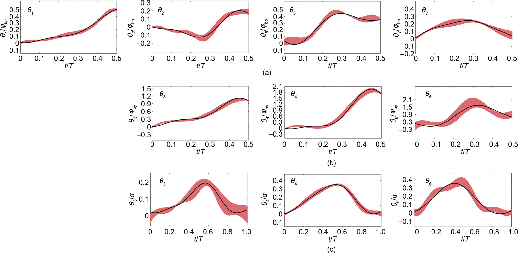
Fig. 10. Joint trajectory curves of the robotic rat. (a) Trajectory curves of pitching joints for B₂, MP₁MP₃, the horizontal axis is the proportion of pitching cycle T and the vertical axis is the proportion of body pitch angle φ_bp; (b) trajectory curves of yawing joints for B₂, MP₂MP₄, the horizontal axis is the proportion of yawing cycle T and the vertical axis is the proportion of body yaw angle φ_by; (c) the trajectory curves of turning joints for B₃, MP₆. The horizontal axis is the proportion of turning cycle T and the vertical axis is the proportion of turning angle α.

Fig. 11 shows the angular velocity of the driving wheel in the turning movement of the robotic rat. The red dotted lines represent the theoretical calculation results, and the black dots represent the value obtained in the simulation environment (ω₁ = 0). The simulation value is close to the theoretical value. Moreover, ω₂ is positively correlated with α and negatively correlated with T.

《Fig. 11》

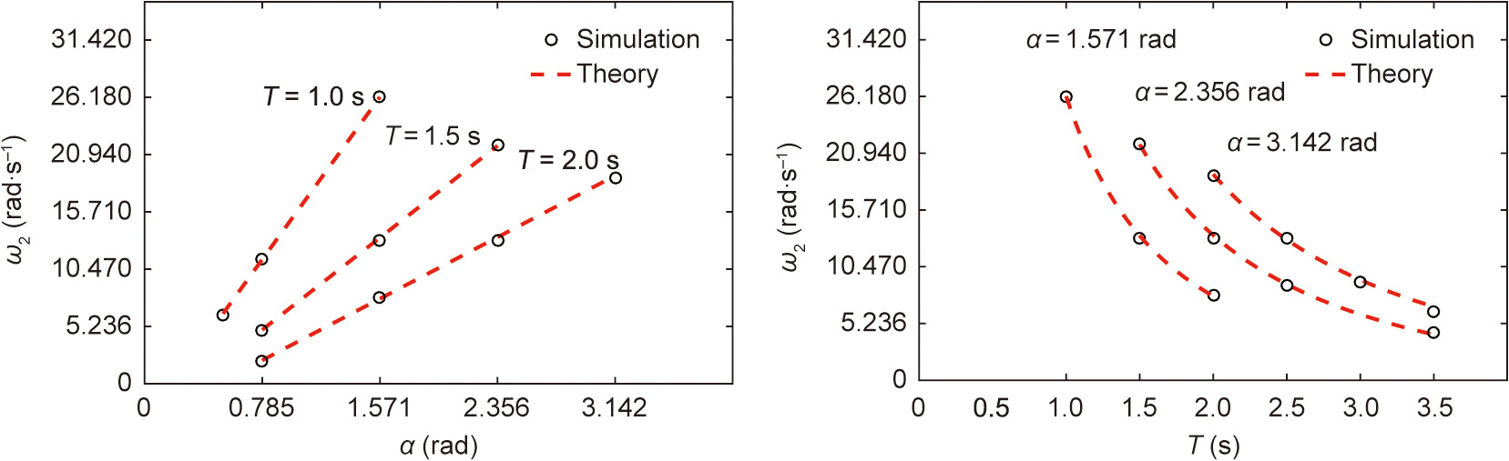
Fig. 11. Angular velocity of the driving wheel.

《3.4. Similarity between the robotic rat and actual rats》

3.4. Similarity between the robotic rat and actual rats

In the simulation and experiment, we first determined the robot the corresponding behavior and combination of MPs based on the obtained behavior-movement hierarchical model. Furthermore, for each combination of MPs, we set its static movement parameters according to the results of clustering analysis. From these static movement parameters, we obtained the generalized trajectory of each joint using the BP neural network. In fact, we have established a robot joint motion library. Once the static movement parameters have been determined, we can obtain the trajectories of each joint using a look-up table. Thus, we obtained the joint state (position, velocity, and acceleration) planned by the robot in advance. In the actual control, we calculated the joint state of the robot in real time and compared it with the preplanned joint state. According to the difference between them, the joint torque was calculated through impedance control, and then each joint of the robot was driven to produce a new joint state. We controlled the robot to produce 50 movements in each group, recorded a total of ten groups, and then calculated the correlation coefficients of various behaviors and movements.

Fig. 12 shows behaviors and movements of the robot over 10 s and the comparison results with the behaviors and movements of actual rats. The results show that the robot has movements that are often relatively similar to those of actual rats. Fig. 13 shows the relationship between correlation coefficient ρ_rat–robot and τ, and c in cluster analysis (taking B₂, MP₁MP₃ as an example). Coefficient τ represents the scale coefficient in hierarchical clustering, which is used to control the density of classification; c represents the number of clusters in FCM clustering. As τ increases, the correlation coefficient first decreases slowly, and then decreases sharply. Here, τ = 0 indicates that each data point is a class, whereas τ = 1 means that all data points are only in one class. When τ = 0, although it has a higher correlation coefficient, the number of samples of the neural network also increases, which increases the training cost of the model. Therefore, we believe that τ = 0.1 is a better choice to reduce the training cost of the model while maintaining a high correlation coefficient. For c, c = 1 and c = n (n = 15, the number of data points) mean that all data points are averaged to obtain the dynamic parameters, which will reduce the correlation coefficient. When c is exactly between 1 to n, the correlation coefficient is higher, indicating that the weighted method is better than the average method. For B₂, MP₁MP₃; c = 3 is a better choice.

《Fig. 12》

Fig. 12. Behaviors and movements of the robot over 10 s.

《Fig. 13》

Fig. 13. Relationship between ρ_rat–robot, τ, and c in cluster analysis.

The correlation coefficients of different behaviors and movements between the robot and rats are shown in Fig. 14. Because the joints of MP₇ and B₅ do not produce displacement, their correlation coefficient was not calculated. Fig. 14(a) shows the movement correlation coefficients during exploration. The sizes of the sectors reflect the observation probability of movements during exploration. The data in every sector are expressed as mean plus or minus standard deviation (SD). Because of the complexity and diversity of head yaw movement in rats, the correlation coefficient of pitching movement (MP₁MP₃) is higher than that of the yawing movement (MP₁MP₂, MP₂MP₄), with a small SD. Fig. 14(b) shows the correlation coefficients of different behaviors. Strongly regular behaviors, such as B₁ and B₆, which only include one repetitive movement, have a higher correlation coefficient and smaller deviation. In contrast, because of the complexity and diversity of combinations in B₃, the correlation coefficient is lower with larger deviation. For more complex and diverse behaviors and movements, more rat data need to be collected and used for training to further improve the correlation coefficients between the behaviors of the robotic rat and rats.

《Fig. 14》

Fig. 14. Correlation coefficients of different behaviors and movements. (a) Movement correlation coefficients in exploration, the sizes of the sectors reflect the observation probability of movements during exploration and the data in every sector are expressed as mean plus or minus SD; (b) correlation coefficients of behaviors, error bars show one SD. SD: standard deviation.

《4. Discussion》

4. Discussion

In the process of behavior classification, we initially divided the behaviors into sniffing, exploring, walking, resting, and grooming. Because of the low correlation coefficient, we subdivided the walking behavior. We made a distinction between continuous straight walking or turning and stop-and-go movement in rats, and matched the four combinations of MPs (MP₅, MP₆, MP₅MP₆, and MP₆MP₅) to the trotting behavior. The above combinations did not include staying (MP₇) and had a relatively quick velocity (Figs. 9(a) and (c)). Next, the behaviors were reclassified, and the movement parameters in walking and trotting were extracted separately. After reclassification, we obtained higher correlation coefficients for the walking and trotting behaviors. Because we only changed part of the original walking behavior into trotting behavior without changing the order of the rat observations, the transition probability between the walking and trotting behaviors is zero when counting the transition probabilities between behaviors. 

Different behaviors and states in the hierarchical model have obvious characteristics. Sniffing is mainly manifested in the movement of repeatedly touching the ground with the tip of the rat’s nose. Exploring is mainly manifested in the pitching and yawing movements of the head and body. Walking is mainly characterized by slower straight and turning speeds, accompanied by short staying periods. In addition, the number of MPs in a combination corresponding to this behavior is usually more than three. Trotting is mainly characterized by faster straight and turning speeds. The number of MPs in a combination corresponding to this behavior is generally no more than two. Resting is mainly manifested by the long staying of rats. Grooming is mainly manifested in the slight head and forelimb movements of rats. The stressed state is mainly indicated by obvious displacement or frequent sniffing and exploring behaviors. The relaxed state is mainly indicated by no obvious displacement, with no movement or only partial, small movements of the head and forelimbs.

Because the limbs of rats rarely move in the reverse direction during the turning movement, we did not drive the robotic rat model in reverse when designing the rotation speeds of the driving wheels to avoid reducing the biomimicry of the robotic rat. At the same time, because of the difference between the wheeled base of the robotic rat and the limbs of rats, the turning radius of the robotic rat is larger than that of actual rats. Under the same driving wheel speed differences, the turning radius of the robotic rat increases substantially as the driving wheel speeds increase. Hence, fixing ω₁ = 0 and only controlling ω₂ to coordinate the motion of the yaw joints in the turning movement is a more reasonable design.

《5. Conclusions》

5. Conclusions

For biomimetic robots, similar behavior models are more conducive to effective interaction between robots and animals. The main focus of this study was to establish the behavior–movement law of rats by extracting different combinations of MPs and corresponding them to different behaviors. The predominant parameters of the MPs were extracted, and the trajectory of each joint was learned and generalized. The correlation coefficient between the robot and rats was used to measure the similarity and control the process of behavior classification and the extraction of movement parameters. A robotic rat model in the ROS environment was used to learn the data and train the robot. The simulation results show that the robot can achieve six typical rat-like behaviors. For each behavior, the robot presents high similarity (the behavior correlation coefficient is greater than 0.8).

In future work, we will implement two modes in the robot: individual mode and interaction mode. In the individual mode, the robot moves based on the law given by the behavior–movement hierarchical model in this paper; in the interaction mode, the robot recognizes the current behavior of the interactive target, and then performs interactive behaviors such as tracking, imitating and contacting. Whether the robot operates in the individual mode or interaction mode will be determined by the interaction probability, that is, the observed probability of interaction between two rats over a series of activities. The behavior and movement of the robot in interaction mode can be further defined on the basis of the approach in this paper. Through interactive control between the robot and rats, we can explore the social behavior mechanism of rats.

《Acknowledgments》

Acknowledgments

This work was supported in part by the National Natural Science Foundation of China (62022014) and in part by the National Key Research and Development Program of China (2017YFE0117000).

《Compliance with ethics guidelines》

Compliance with ethics guidelines

Zihang Gao, Guanglu Jia, Hongzhao Xie, Qiang Huang, Toshio Fukuda, and Qing Shi declare that they have no conflict of interest or financial conflicts to disclose.