
《1. Introduction》
1. Introduction
The discovery, description, and development of Earth’s mineral wealth have long been central pursuits of the Earth sciences. For much of that history, the discoveries of new mineral resources and novel mineral species have been based as much on chance finds as on empirical guidelines. The old adage, ‘‘Gold is where you find it,” has applied to most natural resources, but datadriven discovery is now changing that mantra. In this contribution we review the nature of large and growing mineralogical data resources and describe some of the analytical and visualization methods that are being applied to understand the diversity and distribution of minerals in space and time.
Recent studies fall under three broad headings. Mineral evolution is the investigation of Earth’s changing near-surface mineralogy over 4.5 billion years of history—studies that reveal the striking co-evolution of the geosphere and biosphere and the increasing diversity and complexity of mineral species driven by the chemical differentiation of Earth [1–27]. Mineral ecology, a complementary pursuit, investigates the diversity and spatial distribution of Earth’s minerals, including consideration of the unusual distribution of rare minerals on Earth [28–39]. Finally, mineral network analysis provides a powerful means to analyze and visualize the complex distributions of minerals and their properties through space and time [40]. Taken together, these approaches have the potential to change our view of the evolving mineralogy of Earth and other terrestrial worlds.
《2. Mineral data resources》
2. Mineral data resources
Data-driven discovery relies on comprehensive and reliable tabulations of mineral species, their properties, and their distributions in space and time. The official list of mineral species approved by the International Mineralogical Association (IMA) is documented by the IMA database,↑ which is maintained at the Department of Geosciences, The University of Arizona [41]. In addition to recording more than 5400 mineral species, the RRUFF data resource compiles data on crystal structures, compositions, Raman spectra, and other physical properties. Mineral evolution studies require data on mineral ages, localities, and context—data that is compiled at the Mineral Evolution Database. More than 185 000 individual locality/age data for minerals are available through this rapidly expanding, open-access resource.
↑ https://rruff.info/ima/. ‡ https://rruff.info/evolution
The largest data resource on the global distribution of minerals is mindat.org, ↑↑an international, crowd-sourced effort led by Jolyon Ralph and the Hudson Institute of Mineralogy. The mindat.org data source has recorded more than 1.1 million mineral/locality data from approximately 300 000 localities worldwide—data that are essential in the analysis and visualization of mineral diversity and distribution relationships.
↑↑ https://www.mindat.org.
The essential resources of the IMA database and the mindat.org data source are amplified by a number of other data compilations, most notably the petrological and geochemical resources under the umbrella of the Interdisciplinary Earth Data Alliance (IEDA‡‡), including EarthChem↑↑↑ (e.g., Ref. [42]).
‡‡ https://www.iedadata.org/. ↑↑↑ https://www.EarthChem.org.
An ongoing challenge in developing these critical data resources is the vast amount of ‘‘dark data”—that is, information on mineral compositions, localities, and other data that is available only through hard-copy publications, proprietary corporate documents (notably companies in the natural resources industry), or privately held research records. Data-driven discovery cannot reach its full potential until a culture of data sharing is fully embraced by the Earth science community, with the implementation of ‘‘FAIR” (i.e., findable, accessible, interoperable, and reusable) data practice [43].
Given the rich and growing open-access mineralogical data resources, opportunities for applying a range of powerful analytical and visualization methods beckon [44,45]. In this article, we review a few of these methods as they relate to the fields of mineral evolution, mineral ecology, and mineral network analysis.
《3. Mineral evolution》
3. Mineral evolution
Mineral evolution is the study of the changing near-surface mineralogy of Earth and other terrestrial worlds through deep time [5,19]. Our detailed understanding of Earth’s 4.5-billion-year history of mineralogical change, coupled with a growing understanding of the mineralogy of other solar system bodies [46,47], reveals that a planet’s mineralogy evolves through a sequence of stages, each the result of new physical, chemical, and (in the case of Earth) biological modes of mineral paragenesis.
The greater than 185 000 individual locality/age for minerals tabulated in the mineral evolution database, though far short of recording all available mineral/age information, is sufficiently extensive to reveal striking patterns in Earth’s evolving mineralogy. Three first-order trends stand out.
The first trend in the temporal distribution of minerals is a marked episodicity that reflects the supercontinent cycle of the past 3 billion years [8,12]. We find that Earth has preserved pulses of mineralization during five purported episodes of the convergence and assembly of sometime isolated landmasses into single supercontinents (Fig. 1) [39]. The convergence of continents and consequent orogenic events not only induce mineralization; these mineralizing events are also more likely to be preserved in the cores of the resulting mountain ranges. More detailed investigation of these trends reveals additional subtleties, for example in the unique tectonic and geochemical setting of the assembly of Rodinia at ~1.3 to 0.9 Ga [27].
《Fig. 1》
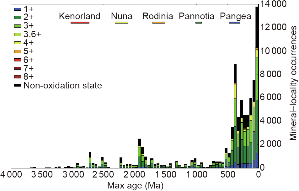
Fig. 1. First-row transition metal mineral–locality occurrences by max age (minerals listed once with highest oxidation state from any first-row transistion elements in formula). Our record of Earth’s minerals through time typically reveals pulses of mineralization that are associated with the supercontinent cycle. In this graph of approximately 60 000 mineral/age data for minerals incorporating firstrow transition metals, pulses of mineralization are associated with the supercontinents Kenorland, Nuna, Rodinia, Pannotia, and Pangea. Note that mineralization associated with Rodinian assembly at ~1.3–0.9 Ga is less distinct than the peaks with other supercontinents, as a consequence of its unique tectonic setting [39]. 1+–8+ refer to different oxidation states.
The second significant temporal trend in Earth’s evolving mineralogy is an observed increase in the average oxidation state of transition metals [20,48]. Thus, for example, the minerals of manganese display a systematic increase in redox state over the past 500 million years, with other fluctuations occurring earlier in Earth’s history (Fig. 2). Similar trends have been observed for all of the redox-sensitive, first-row transition metals (Fig. 3‡‡‡), as well as for uranium [6] and rhenium [20].
‡‡‡ See https://dtdi.carnegiescience.edu for an animated version.
《Fig. 2》
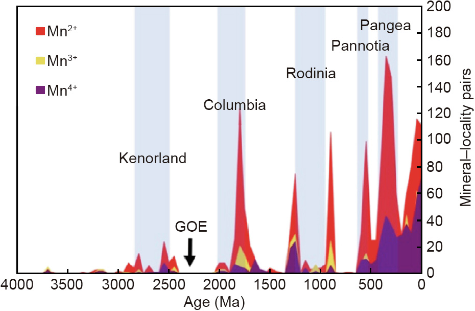
Fig. 2. Changes in Earth’s near-surface oxidation state, the consequence of the evolution of oxygenic photosynthesis, are reflected in the changing ratios of manganese in the II (Mn2+), III (Mn3+), and IV (Mn4+) oxidation states. The average oxidation state of manganese increases, most notably during the past 500 million years. GOE: Great Oxidation Event.
《Fig. 3》

Fig. 3. Normalized mineral–locality occurrences by max age for different elements. A ‘‘skyline diagram” of minerals containing first-row transition elements reveals systematic trends associated with the supercontinent cycle and Earth’s changing atmospheric composition.
The third trend in the evolution of the mineral world is its increasing structural and chemical complexity with the flow of geological time (Fig. 4) [5,11,26]. Numerical estimates of complexity using information-based measures have facilitated the analysis of quantitative correlations between chemical and structural complexities of minerals for a total of 4962 datasets on the chemical compositions and 3989 datasets on the crystal structures of minerals [23,26]. This analysis demonstrates that there is an overall trend of increasing structural complexity with increasing chemical complexity. Moreover, analysis of mean chemical and structural complexities for mineral groups occurring in different geological periods [5,15] has demonstrated that both are gradually increasing in the course of mineral evolution. By analogy with biological evolution [49], the increasing mineral complexity follows an overall passive trend: More complex minerals form with the passage of geological time, yet the simpler ones are not replaced (see also Ref. [35]). The observed correlations suggest that, at a first approximation, chemical differentiation is a major force driving the increase of complexity of minerals throughout Earth’s history. New levels of complexity and diversification observed in mineral evolution are achieved through local concentrations of particular rare elements and the creation of new geochemical environments.
《Fig. 4》

Fig. 4. Mean chemical and structural information-based complexities for minerals occurring in different eras of mineral evolution (1 = 12 ‘‘ur-minerals” [5]; 2 = 60 minerals of chondritic meteorites [5]; 3 = 420 minerals of the Hadean epoch [11]; 4 = all minerals of the post-Hadean era) calculated for a total of 4962 datasets on the chemical compositions and 3989 datasets on the crystal structures of minerals [26]. (a) Shannon information per atom (IG); (b) Shannon information per unit cell or formula unit (IG,total).
《4. Mineral ecology》
4. Mineral ecology
Mineral ecology considers the diversity and spatial distribution of minerals, in much the same way as studies of biological ecosystems document distributions of living species. Earth’s minerals are distributed according to a ‘‘large number of rare events” (LNRE) frequency spectrum, which is common to both biological ecosystems and the distribution of words in a book [29,31,37]. In each instance, a few species or words are extremely common, but most species or words are rare.
Our detailed understanding of distributions of common and rare mineral species is made possible by the mineral/locality data in mindat.org. These data facilitate the calculation of ‘‘accumulation curves,” which reveal estimates of the numbers of ‘‘missing” minerals—those types that occur on Earth but have yet to be discovered and described [28,32]. For example, in a detailed study of the more than 400 carbon-bearing minerals, Hazen et al. [33] predicted that an additional ~145 carbon-bearing minerals await discovery (Fig. 5) [33]. In addition, they listed several hundred candidates for these missing minerals, noting that most would be hydrous carbonates, with a special emphasis on calcium- and sodium-bearing phases that may have been overlooked because they are relatively nondescript—typically white or grey in color and poorly crystallized [32]. This work inspired the Carbon Mineral Challenge,↑ an international project supported by the Deep Carbon Observatory‡ to find as many of the missing carbon-bearing minerals as possible. As of 20 May 2019, at least 30 new carbon-bearing species had been discovered, described, and approved by the IMA.
↑ https://mineralchallenge.net/. ‡ https://deepcarbon.net/.
《Fig. 5》
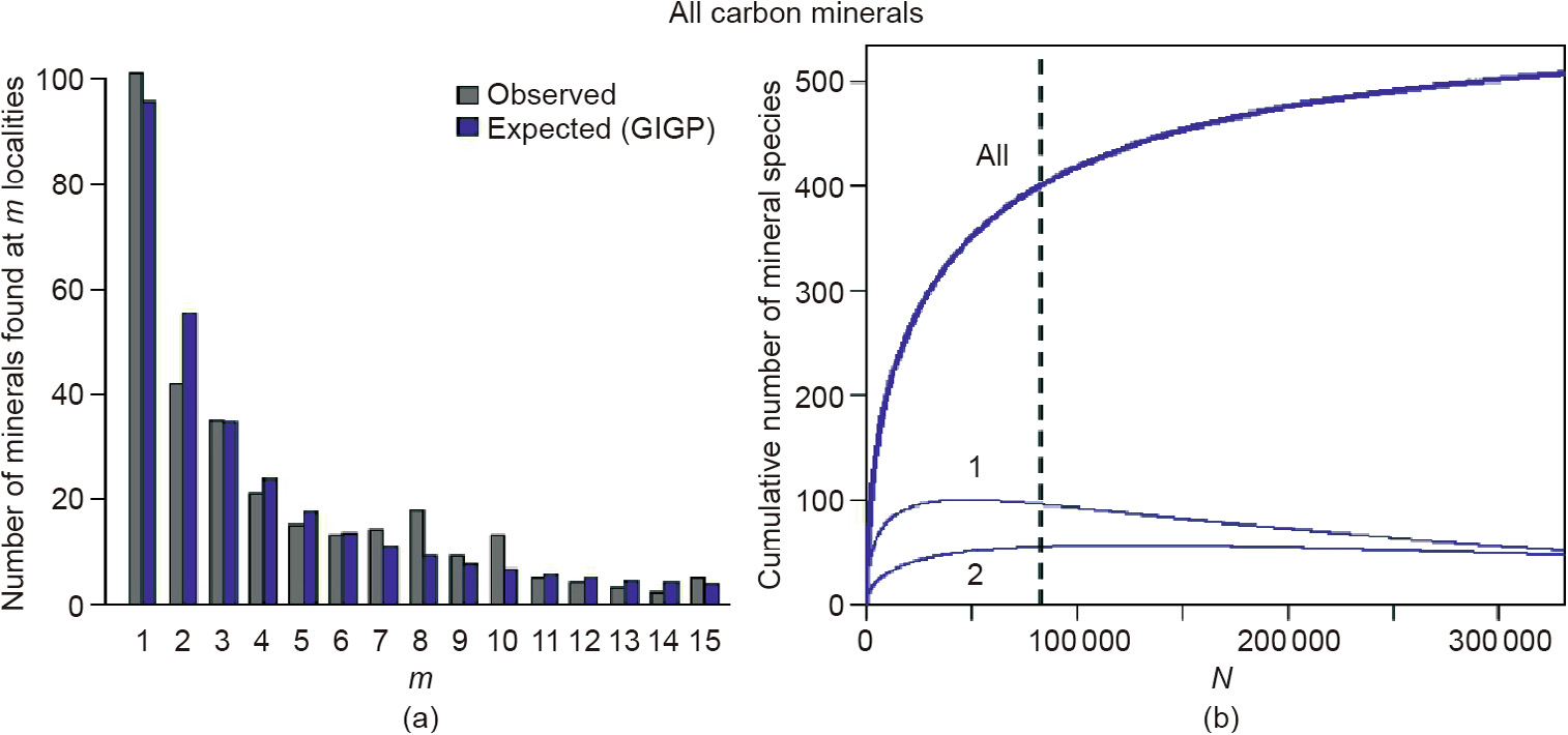
Fig. 5. (a) The frequency spectrum for carbon-bearing minerals reveals that most minerals are rare. The horizontal axis records the exact number of localities (m) at which a carbon-bearing mineral species is found. The vertical axis indicates how many mineral species occur at exactly that number of localities. Grey bars are the observed values, while blue bars indicate the modeled values. Of the 403 documented carbon-bearing minerals in 2016, more than 100 are known from only one locality, while 40 have been described from exactly two localities. (b) This ‘‘large number of rare events” distribution facilitates calculation of an accumulation curve (upper blue curve), shown here on a graph of the number of observed mineral/locality data (N, X axis) versus the estimated number of different mineral species (Y axis). Extrapolation of this curve to the right suggests that an additional 145 carbon-bearing minerals await discovery and description [33]. The vertical dashed line indicates the number of mineral/locality data (82 922) and known species (403) as of 2016. Curves 1 and 2 represent the evolving numbers of different mineral species identified from exactly one or two localities, respectively— values that change systematically as more mineral/locality data accumulate. Note that these curves go through a maximum value; the number of minerals known from only one locality is now declining as more mineral/locality data are reported.
《5. Mineral co-occurrence and network analysis》
5. Mineral co-occurrence and network analysis
One of the most important challenges of mineralogy is to understand the diversity and distribution of minerals in the context of coexisting assemblages of minerals—a problem that requires considering hundreds of species simultaneously. The large and growing mindat.org data resource, coupled with a variety of analytical and visualization methods, is revolutionizing our ability to document these complex multidimensional systems.
《5.1. Chord diagrams》
5.1. Chord diagrams
The first step in any analysis of mineral coexistence is to construct a data object with each mineral species as a separate field. In the simple case of a pairwise mineral co-occurrence matrix, each matrix element represents the number of times that two minerals occur together. These data can be represented by a variety of techniques. Chord diagrams array a group of related mineral species as arcs of a circle, with curved lines connecting coexisting species (Fig. 6). Widely employed in gene analysis, such chord diagrams can also prove useful in mineralogy by illustrating numerous pairwise occurrences in a single visual representation. Chord diagrams can be explored in interactive displays, with embedded metadata on numbers of occurrences, as well as details on localities and other coexisting species.
《Fig. 6》

Fig. 6. A chord diagram of the 43 most common cobalt-bearing minerals reveals coexisting pairs of minerals. This rendering reveals that the secondary mineral erythrite (Co3(AsO4)2·8H2O) is the most abundant cobalt mineral, and that it is most commonly associated with the two most common primary cobalt ore minerals, cobaltite (CoAsS) and skutterudite (CoAs3-x).
《5.2. Klee diagrams》
5.2. Klee diagrams
Klee diagrams (sometimes referred to as ‘‘heat maps”; Fig. 7) also represent the frequency with which pairs of objects—such as minerals or their essential chemical elements—coexist, and thus are a complementary visualization tool to the chord diagram shown in Fig. 6. This method facilitates rapid analysis of coexisting pairs of minerals or elements; however, it is often desirable to understand the associations of more than two objects at a time. Accordingly, Ma et al. [50] have explored the use of interactive three-dimensional Klee diagrams to understand coexisting elements in minerals (Fig. 8). In spite of their potential for quickly revealing occurrence trends among thousands of mineral pairs, Klee diagrams have not yet been widely applied to mineral coexistence relationships.
《Fig. 7》

Fig. 7. Klee diagrams (sometimes referred to as ‘‘heat maps”) represent the frequency with which pairs of minerals, elements, or other objects coexist. This rendering displays a 72 × 72 matrix of coexisting chemical elements in minerals, in which each matrix element represents the fraction of minerals with element X that also incorporates element Y. This matrix is not symmetrical; for example, all minerals containing beryllium also incorporate oxygen, but only a small fraction of oxygen-bearing minerals incorporate beryllium.
《Fig. 8》
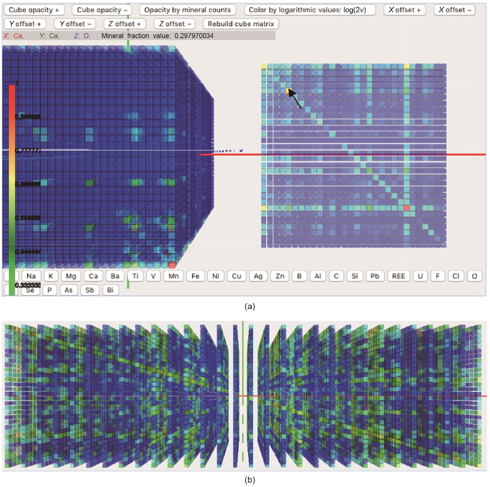
Fig. 8. A three-dimensional interactive Klee diagram facilitates the exploration of triplets of coexisting minerals or elements. This example from Ref. [50] records the frequency of co-occurrence of triplets of chemical elements in minerals. (a) The cube-shaped rendering is difficult to interpret, but any planar slice of the cube can be viewed independently; (b) alternatively, the cube can be rendered in an ‘‘exploded” version to allow users to see the ‘‘inside” of the cube. The red line indicates the centerline of the 3D diagram. The arrow points to one of many ‘‘hot spots,” in this case Ca + Ca + O, where the combination of elements is more commonly found in minerals than would be predicted based on crustal abundances. REE: rare earth elements.
《5.3. Network analysis》
5.3. Network analysis
Network analysis is an especially useful tool for exploring complex interrelationships among numerous mineral species [40]. The use of network graphs to elucidate connections in the contexts of social groups [51–54], technological networks [55–58], and biological systems [59–62] are well known. Each network consists of vertices (or nodes), some of which are connected to each other by edges (or links). Distances between nodes, and hence the length of links, are determined by the degree of association of the two nodes; shortest distances represent the strongest links. Vertices and edges can be sized, shaped, and colored to indicate additional attributes of the system.
Networks of coexisting minerals provide vivid examples of network graphs.↑ In Fig. 9 [40], individual nodes represent mineral species. The nodes are sized to represent the relative number of localities of each species, while node colors can represent compositional, structural, paragenetic, or other information. These highly interactive visual displays represent projections from multidimensional space into two- or three-dimensional space, in order to show the connections from each mineral node to all other co-occurring mineral nodes. In general, for a well-connected network of N different mineral species, the rendering is a projection from N – 1 dimensions. In many instances, a three-dimensional rendering provides important additional information, even though the projection may be from much higher dimensions.
↑ See https://dtdi.carnegiescience.edu for interactive examples.
《Fig. 9》

Fig. 9. Network graphs of mineral species. (a) 58 chromium-bearing minerals: nodes are sized according to mineral frequency of occurrence, and colored according to mode of formation (see inset). This low-density network shows strong clustering based on paragenetic mode. (b) 664 copper-bearing minerals: nodes are sized according to mineral frequency of occurrence; nodes are colored according to the presence or absence of S or O (see inset; after Ref. [40]).
Network graphs not only represent local properties—such as all of a given mineral’s coexisting species—but they also reveal global trends not easily discerned from the data alone, such as clustering by chemistry or paragenetic mode, the degree of a network’s interconnectedness, and otherwise hidden compositional and temporal trends. A distinct advantage of network statistical analysis is the opportunity for network metrics that characterize global and local statistical properties of the network [63,64]. Metrics, including density, centrality, and diameter, facilitate the comparison of related networks, such as those representing minerals incorporating different chemical elements or a time series for minerals of a given element [40].
《5.4. Bipartite network graphs》
5.4. Bipartite network graphs
Several rendering options exist for network graphs. Of special importance to mineralogy are bipartite graphs [65], which can display two distinct types of nodes, such as representing both mineral species and their localities (Fig. 10). A striking feature of mineral bipartite networks—one not reported from such graphs of other natural or artificial systems—is the distribution of locality nodes in a ‘‘U-shape” (or ‘‘vase shape” in three dimensions), with fewer very common minerals inside the U (or vase), and many more rare minerals decorating the periphery (Fig. 10). This distribution is a visual representation of an LNRE spectrum, with relatively few very common minerals and numerous rare species.
《Fig. 10》
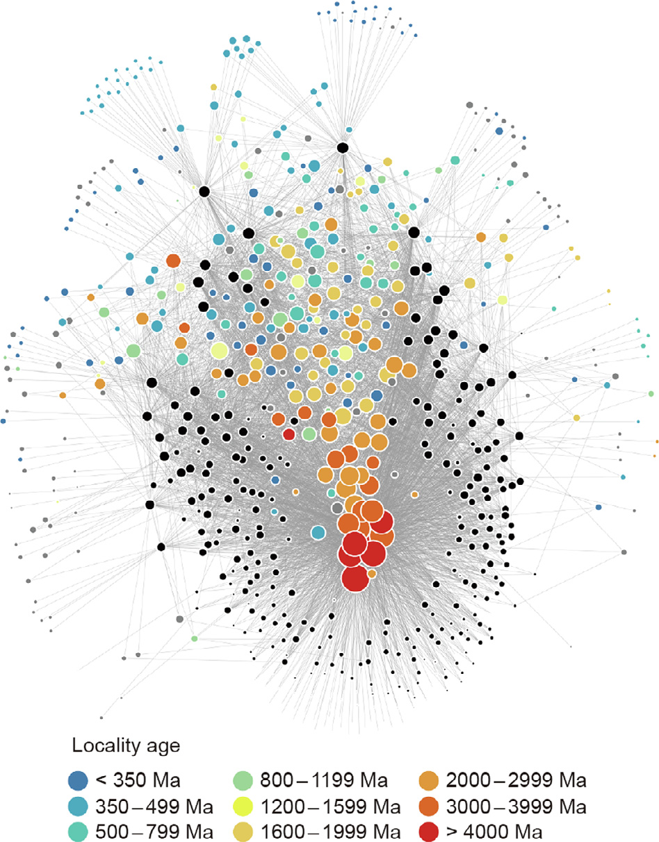
Fig. 10. Bipartite network of 403 carbon-bearing mineral species. Colored circles represent carbon mineral species, with circle sizes representing relative frequency of occurrence and colors (see inset scale) corresponding to the age of earliest known occurrences of those minerals. Black circles represent regional localities, with sizes corresponding to the relative numbers of different carbon-bearing minerals found at those localities. The network rendering reveals important information regarding the diversity and distribution of carbon minerals through space and time. In particular, the ‘‘U-shaped” distribution of black locality nodes, with a few very common carbon minerals ‘‘inside” and many more rare carbon minerals ‘‘outside,” is an alternative visual representation of the LNRE distribution illustrated in Fig. 5. Note that most of the common minerals are more ancient, whereas most of the rare minerals are more recent. See also http://dtdi.carnegiescience.edu/node/4557 for an interactive version.
《6. The future》
6. The future
Data-driven discovery in mineralogy is still in its infancy. Openaccess mineral data resources need to be expanded by at least an order of magnitude, with a special effort made to recover dark data that will otherwise be lost. New analytical and visualization methods, some tailored specifically to mineralogy, must be created and implemented. In addition, opportunities will emerge to apply these methods to other terrestrial planets and moons, as data from Mars, the moon, and other worlds are gathered.
A critical need is to merge a variety of databases with a deeptime component and correlate their various data fields. Efforts are underway to correlate mineralogical databases to other deeptime databases, such as geochemical, paleontological, and protein databases, in order to gain a more holistic picture of the coevolution of Earth’s geosphere and biosphere.↑ These studies have the potential to reveal how Earth’s changing near-surface mineralogy and geochemistry have influenced the biochemistry of organisms, and how life, in turn, created new mineral species and geochemical niches.
↑For example, https://dtdi.carnegiescience.edu.
《6.1. Affinity analysis》
6.1. Affinity analysis
Perhaps the most exciting prospect is the targeted discovery of new mineral occurrences, including new economically valuable resources, employing the methods of affinity analysis. A taste of what is to come was provided by a recent prediction by Jolyon Ralph of mindat.org (personal communications, May 2018). Using only pairwise mineral correlations, Ralph predicted that the uncommon mineral wulfenite (PbMoO4) should occur at Cookes Peak, New Mexico, a lead–zinc–silver mining district with more than 75 reported mineral species but lacking reports of wulfenite. Subsequent scrutiny by local mineral collectors revealed pockets of this beautiful, but previously overlooked, mineral.
Affinity analysis (also known as ‘‘market-basket analysis” when applied to product recommendations by online companies), employs a similar approach but with multidimensional positive and negative co-occurrence information [66–68]. Initial trials of affinity analysis to minerals will expand search algorithms beyond pairwise coexistence data to larger combinations of characteristic mineral species. In the near future, we hope to interrogate mindat.org to compile lists of ‘‘missing” minerals with their probabilities of occurrence at known localities—a testable approach to the development of predictive mineralogy.
An aspiration of our program is to search for mineral and other natural resources by applying affinity analysis to expansive data resources that include numerous fields related to mineral occurrences, their chemical compositions (including trace-element and isotopic data), and physical properties, as well as the physical, chemical, and biological environmental context of those mineralized occurrences. We anticipate that recommender systems will play a key role in the next generation of natural resource exploration.
《6.2. Crystal chemical systematics》
6.2. Crystal chemical systematics
Data-driven efforts by Gagné and Hawthorne [69–72] and Gagné [73] have recently provided a baseline statistical knowledge of the bonding behavior of atoms in oxide, oxysalt, and nitride crystals. This congregated knowledge, soon to be expanded to sulfide and sulfosalt minerals, allows prediction of the most likely composition of ‘‘missing minerals” in a much more precise way by combining knowledge of the ideal bond valences of a crystal structure [74] and the ability of the ions to adopt predicted bonding requirements. This influx of organized bonding data further allows the derivation of high-quality bond-valence parameters (e.g., Ref. [75]), which are useful in the context of mineral evolution to better infer the oxidation state of redox-sensitive transition metals in studying Earth’s changing near-surface environments.
《7. Conclusions》
7. Conclusions
Data-driven discovery in mineralogy represents one aspect of the dynamic ‘‘open data movement” that has the potential to change the pace of scientific discovery [76,77]. Progress will depend on parallel advances in building comprehensive data resources, developing and implementing advanced analytical and visualization methods, and applying these capabilities to outstanding mineralogical problems. In some cases, these data science methods will accelerate hypothesis-driven science by enhancing our understanding of the diversity and distribution of minerals— findings that we know we don’t know. Even more exciting is the prospect that multidimensional analysis of mineral systems will lead to the abductive discovery of new and unexpected insights— discoveries of what we didn’t know we didn’t know.
《Acknowledgements》
Acknowledgements
We are grateful to Ho-Kwang Mao and the organizers of this special issue for the opportunity to share our results. This publication is a contribution to the Deep Carbon Observatory.
Studies of mineral evolution and mineral ecology are supported by grants from the Alfred P. Sloan Foundation (G-2016-7065), the W. M. Keck Foundation (grant entitled ‘‘Co-Evolution of the Geosphere and Biosphere”), the John Templeton Foundation (60645), the NASA Astrobiology Institute (1-NAI8_2-0007), a private foundation, and the Carnegie Institution for Science. Sergey V. Krivovichev acknowledges support from the Russian Science Foundation (19-17-00038).
《Compliance with ethics guidelines》
Compliance with ethics guidelines
Robert M. Hazen, Robert T. Downs, Ahmed Eleish, Peter Fox, Olivier C. Gagné, Joshua J. Golden, Edward S. Grew, Daniel R. Hummer, Grethe Hystad, Sergey V. Krivovichev, Congrui Li, Chao Liu, Xiaogang Ma, Shaunna M. Morrison, Feifei Pan, Alexander J. Pires, Anirudh Prabhu, Jolyon Ralph, Simone E. Runyon, and Hao Zhong declare that they have no conflict of interest or financial conflicts to disclose.


 京公网安备 11010502051620号


