

《1. Introduction》
1. Introduction
The shortage of freshwater has become a significant problem for humanity, given the continuously increasing world population and developing industry [1]. Compared with other technologies, including multi-effect distillation, multi-stage flash distillation, and vapor compression distillation, reverse osmosis (RO) technology is recognized as an effective tool to mitigate this problem, mainly due to its lower energy consumption [2]. However, RO technology has its own bottlenecks, which include the tradeoff effect between water flux and ion rejection. Hence, researchers have made efforts to design new membranes that can maximize water flux without sacrificing ion rejection [3]. Since the first commercial composite RO membranes were developed in the 1970s [4], a great deal of progress has been made in enhancing their performance, mainly by optimizing the structure and chemistry of the separation layers [5]. However, it seems difficult to noticeably improve the water flux without sacrificing ion rejection using only the empirical knowledge gained over the past decades [6]. To tackle this problem, it is necessary to have a deeper understanding of the mechanism of the ion rejection and water transport through RO membranes at the molecular level. Compared with experimental methods, molecular dynamics (MD) simulation offers a powerful way to observe the particle motions in nanoconfinement [7].
Flat-sheet RO membranes typically possess a thin-film composite structure consisting of three layers: an ultra-thin separation layer, a porous interlayer, and a non-woven substrate. The ultrathin separation layer determines the permeability and selectivity of RO membranes; thus, most MD simulations have focused on this layer. For example, the physical properties of RO membranes were first studied via MD simulations [8–11]. Researchers have also paid intense attention to the effect of the structure of the separation layer on the water flux, as well as to the molecular mechanism of water passing through this layer. Ding et al. [12] simulated the process of water passing through RO membranes, and found that water molecules confined in the membrane formed an interconnected hydrogen-bond network made of cyclic and linear aggregates. Gao et al. [13] confirmed that the non-equilibrium condition of RO membranes can be simulated by non-equilibrium molecular dynamics (NEMD) simulations. Shen et al. [14] further observed that water transport is promoted with an increasing fraction of connected percolated free volume. Luo et al. [11] used equilibrium MD simulation to predict ion rejection from the free energy and ion paths. In these simulations, a hydrated membrane with outside water/solution reservoirs was usually used. This model is typically very successful in describing the whole transport process. Moreover, the results from these simulations have offered meaningful guidance in changing the chemical structure of the monomers and the polymerization process for better performance. However, these simulation works did not distinguish between the interfacial resistance and the interior resistance out of the total resistance for the RO process, which would result in unreliable estimation and prediction of the experimental water flux.
When water molecules pass through RO membranes, transport resistance is produced by two parts: namely, water molecules entering into and exiting from the membrane (interfacial resistance); and water being transported inside the membrane (interior resistance) [15]. Hence, the resistance from these two parts should be dealt with separately, since only interior resistance is related to the membrane thickness, and only this part should be multiplied when estimating the water flux under experimental conditions (introduced in detail in Section 2.1). To obtain the interfacial and interior resistances separately, two models need to be built: one with water reservoirs, and the other without water reservoirs. The model without water reservoirs describes the behavior of water flowing inside the membrane, and can be used to obtain the interior resistance directly. The total resistance can be obtained using the model with water reservoirs, as this model describes the whole process, including the water molecules entering into and exiting from the RO membrane and the transport of water molecules inside the RO membrane. After separately obtaining the total resistance and the interior resistance from the simulations, the interfacial resistance can be obtained by subtracting the interior resistance from the total resistance. Then the pure water flux under experimental conditions with a thickness greater than 100 nm can be estimated by multiplying the interior resistance (rather than the total resistance) by the factor of membrane thickness, and then adding the interfacial resistance to obtain the total resistance of the membrane in the experimental condition.
In this work, we applied steady-state non-equilibrium molecular dynamics (SS-NEMD) simulations in order to investigate the resistance distributions of membranes with various hydrophilicities, by directly applying external forces (EFs) on the oxygen atoms of water molecules. After performing the SS-NEMD simulations, the resistances were calculated and the water flux under experimental conditions was then estimated. By separating the interior and interfacial resistances, we investigated the relationship between the hydrophilicity and resistance. Furthermore, in order to confirm the reliability of our proposed method, the simulated water flux and ion rejection for polyamide (PA) RO membranes with various compositions were compared with experimental results from an earlier published study [16].
《2. Methods》
2. Methods
《2.1. Resistance contributions of PA RO membranes》
2.1. Resistance contributions of PA RO membranes
Simulation results are usually compared with experimental outcomes directly. However, due to the limitation of computational capabilities, the thickness of membranes in simulations is quite small (5–10 nm) compared with the real thickness used in experiments (> 100 nm). Thus, the resistances from simulations are usually estimated by considering the factor of thickness and the water flux, as described by Eq. (1):


where J is the pure water flux,  is the pressure drop, μ is the water dynamic viscosity, R is the transport resistance, and d is the membrane thickness.
If only one model (with water reservoirs) is applied, it is not possible to distinguish the interfacial and interior resistances from the total resistance (Rinterfacial + Rinterior) of the membrane. Consequently, the interfacial resistance is unexpectedly multiplied during the estimation process using Eq. (1b). Hence, it is necessary to distinguish between the interfacial resistance and the interior resistance, as described in Eq. (2):
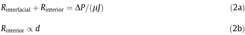
where Rinterfacial is the interfacial resistance, and Rinterior is the interior resistance. It is obvious that only Rinterior is proportional to the membrane thickness.
《2.2. Construction of the RO membrane》
2.2. Construction of the RO membrane
The dependence of resistance on the composition of PA RO membranes is also of concern, because understanding this dependence will help in the design of high-performance PA RO membranes. Our previous work [17] demonstrated that the residual carboxyl groups in the PA separation layer had a strong affinity to the water molecules, resulting in higher water transport resistance. The typical interfacial polymerization between trimesoyl chloride (TMC) and m -phenylenediamine (MPD) does not offer much flexibility to tune the chemistry of the resulting PA layer. Therefore, in this work, we chose two types of acyl halide monomers to construct our PA RO membranes: biphenyl tetraacyl chloride (BTEC), with four acyl halide groups, and isophthaloyl dichloride (IPC), with two acyl halide groups. By adjusting the ratio of BTEC and IPC, the content of residual carboxyl groups can be easily tuned. In this way, the dependence of transport resistance—especially the separated interior resistance and interfacial resistance—on the composition of PA RO membranes can be unveiled. As discussed above, each membrane of a certain hydrophilicity was applied in simulations of two models: one with water reservoirs and the other without.
We performed SS-NEMD simulations with the large-scale atomic/molecular massively parallel simulator (LAMMPS) program [18]. The atomic interaction was modeled with the polymerconsistent force field (PCFF), which is suitable for polymers and inorganic materials [19]. The total potential energy (Etotal) of a system can be defined as shown in Eq. (3):

where Evalence comprises bond stretching, angle, torsion, and out-of-plane energies, while Ecross-term includes bond length and angle changes. Non-bond energies (Enon-bond) are divided into Lennard– Jones (LJ) (9–6) van der Waals and Coulombic interactions [20,21]. The water model is also described by the PCFF.
Following our previous work [17], we expected to compare the resistance of water molecules entering into (and exiting from) membranes with the resistance of water flowing inside membranes in this work. Therefore, we constructed membranes with and without water reservoirs, in order to calculate the total resistance and the resistance inside the membranes, respectively. The monomers 3,3' ,5,5' -BTEC, IPC, and MPD that were used in our simulation—and that are identical to those used in the experimental work of Zhao et al. [16]—are shown in Fig. 1. The polymers were first composed with 500 MPD units, n BTEC units, and m IPC units, and were randomly positioned in a 5.5 nm × 5.5 nm × 5 nm rectangular box to reach the proper density [22]. The repeat units of the polymers were linked by forming amide bonds through the reaction between –COCl and –NH2 groups. Therefore, we bridged –COCl on one end and –NH2 on the other on the basis of an heuristic distance criterion [23]. A total of 1600 water molecules were inserted into the system to maintain a water content of 23% [10]. After that, energy minimization was performed to make the molecules spread homogeneously. Moreover, unreacted –COCl groups were artificially transformed to –COOH groups to form the final membranes without water reservoirs.
《Fig. 1》
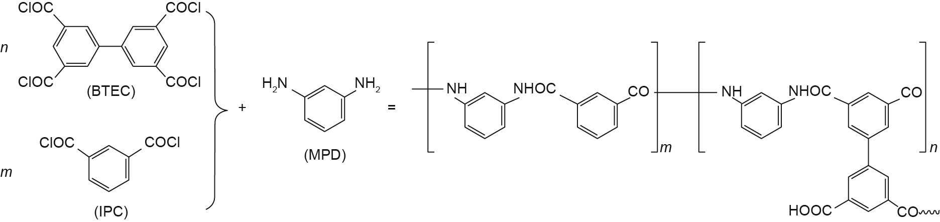
Fig. 1. The chemical equation of the polymerization of BTEC and IPC with MPD to produce PA.
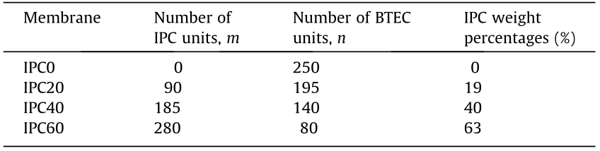
Four membranes with different ratios of BTEC and IPC were made using the same modeling method described above. To ensure that the various membranes had the same thickness and density, we constrained the simulation boxes in the same size. The compositions of these four membranes are listed in Table 1, in which the IPC weight percentage is calculated by dividing the mass of the IPC by the total mass of acyl halides. To obtain membranes with water reservoirs, an additional 2000 water molecules were placed on both sides of the hydrated membranes. On the left side, 40 sodium (Na) ions and 40 chlorine (Cl) ions were solvated by water molecules to imitate seawater [24]. Periodic boundaries were applied in all three directions. After energy minimization, the system was performed as an isothermal–isobaric ensemble (NPT ) at 300 K and 0.1 MPa in the z direction for 1 ns to obtain a correct water density. The final configuration is shown in Fig. 2. The SS-NEMD simulations were then performed.
《Table 1》
Table 1 Compositions of the PA membranes with various IPC contents.
《Fig. 2》
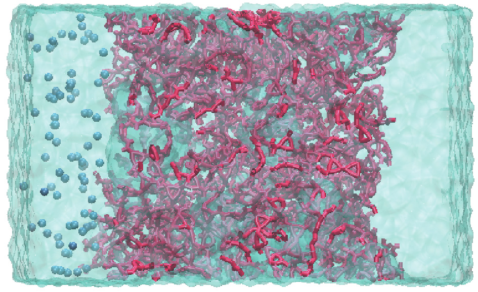
Fig. 2. A snapshot of the final configuration of hydrated PA (with water reservoirs). PA atoms are marked in red and ion particles are represented in blue.
It should be noted that this method is only valid provided that the structure of the membranes is homogeneous. In this simulation, we applied periodic boundary conditions in all three directions, and the model we built is actually a reduced-scale representation of the experimental PA membrane. Hence, the simulated model can be seen as a homogeneous structure while predicting the experimental thickness of the membrane.
《2.3. Details of SS-NEMD simulations》
2.3. Details of SS-NEMD simulations
NEMD simulation is a technique to explore fluid transport through porous media [25,26]. There are two ways to achieve pressure gradients: One is by applying an EF on the particles, and the other is by using movable walls (MWs) as pistons [27]. With the EF method, the pressure drop can be related to the constant applied force on each water molecule. One of the advantages of this method is that it allows researchers to discover the dynamics properties inside the membrane without liquid reservoirs, which can prevent the influence of interfacial effects on water dynamics [17,28]. A modified EF approach was proposed by Ritos et al. [29] and Borg et al. [30], who imposed a pressure difference between the two reservoirs by applying a Gaussian-distributed force over cross-sectionally uniform areas only. This approach is very suitable for the simulations of complex geometries, especially for the cases with a non-uniform cross-sectional area, which produces constant pressure drops. With the MW method, the pressure drop is produced by applying a large force on the upstream wall and little force on the downstream wall. In fact, this method also makes it possible to maintain constant pressures, but it breaks the periodicity in the flow direction.
We used molecular simulation to calculate the total transport resistance by dividing it into two contributions: the interfacial part and the interior part. Hence, it was necessary to build a molecular model without outside reservoirs. For the model excluding water reservoirs, adding forces on all water molecules is the only way to generate pressure drops. In addition, the hydraulic permeability of RO PA membranes is extremely low, such that it might be difficult to just apply forces outside the polymer membrane to carry out NEMD simulations. Moreover, Ding et al. [31] have validated this method, so that the simulated values were in good agreement with the experiment. In this work, we applied the EF on fluid atoms, which included water molecules and ions, in order to mimic the pressure drop. To hinder spurious rotational dynamics, an EF was applied to the water oxygen atoms instead of to the water molecules themselves [31]. When we measured the transport properties, we tracked the positions of fluid atoms passing through the membrane during the simulation time. Since threedimensional periodic conditions were applied in our simulations, there was no clear boundary for the feed and permeate sides. Hence, the ion rejection was determined by counting the number of ions passing through the PA membrane regions. The pressure drop simulated here was two orders magnitude higher than the experimental one. This is because a small force led to a low signal-to-noise ratio; thus, an extremely long simulation was needed to obtain a small uncertainty while measuring the streaming motion, leading to a tremendously large computational cost.
The temperature of the PA membrane was regulated using a canonical ensemble (NVT ) at 300 K. As mentioned above, we added forces on the water molecules that would result in a constant energy input. In order to prevent unexpected rising of the water temperature, the temperature of the water was thermostated at 300 K based on the temperature excluding the center-of-mass velocity, which is widely applied in NEMD simulations [32]. The temperature results as a function of the simulation time of IPC0 with water reservoirs are provided as an example in Appendix A Fig. S1. The reason for the steady temperature is that the additional energy can be removed well through this method.
We applied forces (Fz ) of 0.1722, 0.1865, 0.2000, 0.2152, and 0.2296 kcal·mol-1 Å-1 (1 kcal = 4184 J) on water molecules in cases without water reservoirs and forces of 0.0492, 0.0533, 0.0574, 0.0615, and 0.0656 kcal·mol-1 Å-1 in cases with water reservoirs in order to generate different pressure drops (600, 650, 700, 750, and 800 MPa) along the z direction. To constrain the water flow along the z direction due to the force exerted by flowing water molecules, and to maintain the flexibility of the PA as much as possible, we pinned a few PA atoms that were uniformly distributed in the system during the simulations [14]. The simulations were performed for 7 ns, where the data from the first 2 ns were allowed to reach the steady state and were not used for further analysis. The trajectories were gathered by saving data every 10 000 steps with a time step of 1 fs. After the whole simulation process, we used the trajectories to analyze the structural and dynamics properties of water molecules in the RO membranes.
《3. Results and discussion》
3. Results and discussion
《3.1. Structural properties of the membrane》
3.1. Structural properties of the membrane
Since the structural properties certainly influence the dynamic properties of water molecules in the RO membrane, it is necessary to figure out whether the structural properties of RO membranes are dependent on the monomer compositions. The densities of the water reservoirs and hydrated membranes were first investigated, and are shown in Fig. 3.
It is obvious that, for all cases, there are three regions: bulk water regions, the polymer/water interfacial regions, and the interior regions of the hydrated membrane. The water density stays at around 1 g·cm-3 in the bulk water regions, then drops sharply at the polymer/water interface, and finally reaches about 0.24 g·cm-3 within the interior regions. Such findings are consistent with the results of published simulation works [17,33]. The formation of the polymer/water interface contributes to the swelling of the PA. In the interior regions, the oscillation in density within a reasonable range is influenced by the presence of voids inside the membrane. From Fig. 3, it is obvious that the density profiles of the PA are not exactly the same from case to case. This phenomenon is derived from the various distributions of water clusters in the PA membranes. Although the density profiles are slightly different, they have almost the same average density (about 1.24 g·cm-3 ) for hydrated PA.
It should be noted that the interfacial width of Fig. 3(a) is obviously wider than those of the other three membranes, indicating a higher degree of swelling for the IPC0 case. This higher degree of swelling may stem from the more hydrophilic nature of IPC0. Meanwhile, a higher degree of swelling might reduce the interfacial resistance because of the higher water content. To verify this higher degree of swelling for IPC0, a 10 nm-thick IPC0 membrane was also constructed. The density distribution is shown in Appendix A Fig. S2, which represents a similar degree of swelling.
《Fig. 3》

Fig. 3. The densities of PA and water molecules as a function of membrane position in the z direction (the direction of the membrane thickness) for membranes with various IPC contents: (a) IPC0, (b) IPC20, (c) IPC40, and (d) IPC60. “Dry polyamide” represents the density of PA atoms excluding the water molecules around them.
To further confirm that these four membranes have similar interior pore sizes, we calculated their pore size distribution (PSD). The PSD was measured by a Poreblazer v3.0, which incorporates a Monte Carlo Integration procedure described elsewhere [34]. The PSD of each membrane is shown in Fig. 4. The pore diameter is almost within the range of 4–10 Å for all membranes. As the pore is formed by the PA and is filled with water molecules, the minimum pore size must be larger than the diameter of a single water molecule (about 3.2 Å). The maximum pore size is less than 10 Å, which falls in the range of the average pore sizes of the PA RO membrane [35].
The statistics of the average pore size of each membrane are also shown in Fig. 4. In Figs. 4(a) and (c), the pore sizes are welldistributed, because the proportions of each pore size are basically the same. In Fig. 4(b), the pore sizes of 0.65 and 0.95 nm occupy a peak section. In Fig. 4(d), the pore sizes mostly distribute from 0.6 to 0.7 nm. Although the distributions of the pore sizes differ from each other, it is clear that the average pore size of each membrane is around 0.72 nm, which is calculated as the integration of the PSDs. The average pore sizes are closely consistent with the pore diameter of RO membranes—about 0.70 nm, as estimated by other research [36]. As the water flux is almost linear with the square of the pore radius [37], the similar pore size for each membrane ensures that the transport resistance contributed by the factor of pore size is almost the same for membranes with various IPC contents. Furthermore, the average pore size of 0.72 nm allows the membranes to permeate water molecules and hinder the passage of ions [38]. The permeation of water and the ion rejection properties of the four membranes will be discussed below.
《Fig. 4》

Fig. 4. PSDs of membranes with various IPC contents: (a) IPC0, (b) IPC20, (c) IPC40, and (d) IPC60.
《3.2. Pure water flux》
3.2. Pure water flux
Five pressure drops (600, 650, 700, 750, and 800 MPa) were generated to determine the dynamic properties of water molecules passing through the membranes. It is obvious that the water flux is almost proportional to the pressure drops, despite small fluctuations due to random thermal motion. Thus, the water flux at lower pressure drops, such as under the experimental conditions of 5.5 MPa, can be directly estimated [14].
For each case of monomer composition, we applied two models: with and without water reservoirs. From the model with water reservoirs, the total resistance can be calculated using Eq. (2a). The interior resistance can be calculated from the model without water reservoirs as well. Next, it is possible to calculate the interfacial resistance by subtracting the interior resistance from the total resistance. From Fig. 5(a), the slopes are 370 and 140 for the cases without and with water reservoirs, respectively; the interior and interfacial resistance can then be calculated, as shown in Fig. 6.
《Fig. 5》

Fig. 5. Water fluxes of membranes with various IPC contents: (a) IPC0, (b) IPC20, (c) IPC40, and (d) IPC60.
《Fig. 6》

Fig. 6. Simulated resistances of the membranes (thickness = 5 nm) with various IPC contents.
When the IPC content increases, the slope for the cases without water reservoirs rises to 491, while the slope for the cases with water reservoirs drops to 123. For the cases without water reservoirs, the rising slopes indicate promoted permeability and lower interior resistance. For the cases with reservoirs, the dropping slopes indicate reduced permeability and higher total resistance.
《3.3. Analysis of transport resistance》
3.3. Analysis of transport resistance
According to Eq. (2), it is possible to directly obtain the interior resistance and total resistance after obtaining the relationship between the water velocity and the pressure drop with two distinct models. The interfacial resistance was obtained by subtracting the interior resistance from the total resistance, because the membranes with or without water reservoirs have the same membrane thickness in our simulations. After that, the interior and interfacial resistances at the simulation thickness can be calculated. The interior resistance at the experimental thickness can be calculated by multiplying the thickness coefficient (i.e., the thickness ratio between the membranes used in real experiments and those used in the simulation) with the simulated interior resistance. Finally, the total resistance at the experimental thickness is obtained by determining the sum of the interfacial resistance and the equated interior resistance at the experimental thickness. It is worth mentioning that this process is reliable because of the assumption that the membrane thickness has a negligible effect on the interfacial resistance [39]. Fig. 6 shows the simulated resistance for a membrane thickness of 5 nm.
Since each BTEC unit leaves behind some residual carboxyl groups after polymerization with MPD while the IPC unit does not, an increase in IPC content will lead to a decreased number of residual carboxyl groups in the produced PA separation layer. Our previous work [17] demonstrated that the carboxyl groups in the PA separation layer had a strong affinity to the water molecules. Hence, fewer carboxyl groups will attract fewer water molecules, so that the interior resistance of the water molecules will be diminished. The results of the calculated resistance in this work confirmed this conclusion again. As shown in Fig. 6, with increasing IPC content (which means decreasing BTEC), the interior resistance keeps dropping.
The change in the interfacial resistance is opposite to that in the interior resistance. While the IPC content increases, the interfacial resistance rises obviously, which is in accordance with most MD simulation work [24]. This phenomenon originates from the strong affinity between carboxyl groups and water molecules. Fewer carboxyl groups remaining on the surface of the PA layer attract fewer water molecules, resulting in poor wetting of water molecules to the membrane surfaces and, consequently, a greater interfacial resistance.
Moreover, Fig. 6 reveals that the interfacial resistance amounted to more than 62% of the total resistance for various IPC contents, indicating that the membrane thickness, which determines the interior resistance, plays a less important role in influencing the total resistance of the RO membranes. These simulations are based on PA layers with a thickness of 5 nm; however, the PA layer of a real RO membrane typically has a thickness of about 200 nm. To estimate the resistance of real RO membranes, a typical method is to multiply the resistance of the 5 nm PA layer by a factor of 40, based on the difference in thickness. This method is reasonable in regards the interior resistance, which is merely dependent on the distance of water transport inside the membrane—that is, on the thickness of the PA layer.
The interfacial resistance, which is determined by the surface properties, does not change with the thickness of the PA layer. Therefore, such a method will significantly overestimate the interfacial resistance, and correspondingly overestimate the total resistance. Based on this unreliable method, it may be concluded that the interfacial resistance also plays a dominant role in the total resistance of RO membranes, as the ratio of interior and interfacial resistance does not change with the thickness of the PA layer in this simple estimation. Such a finding is obviously inconsistent with experimental observations, where thinner PA layers always lead to greater water permeability [40–42].
In order to further validate the method of estimating the experimental water flux of the RO membrane, a membrane was constructed with water reservoirs at a length of 10 nm and with IPC0 contents. Similarly, five pressure drops (600, 650, 700, 750, and 800 MPa) were applied on the membrane. The relationship between water flux and pressure drops is shown in Fig. S3. The slope is about 98, from which it can be calculated that the water flux is about 539 L·m-2 h-1 at 5.5 MPa. From Eq. (2), it is possible to estimate the water flux at a thickness of 10 nm, based on the results of the 5 nm case; this is 559 L·m-2 h-1 . That is, the error is only 3.7%, which validates the estimation process proposed in Section 2.1.
Alternatively, the resistance of a real RO membrane with a 200 nm PA layer can be estimated by separately considering the interfacial and interior contributions. The interfacial resistance remains unchanged compared with that of the 5 nm PA layer, while the interior resistance of the 5 nm PA layer is multiplied by a factor of 40 to obtain that of the 200 nm PA layer. As shown in Fig. 7, the interior resistance now plays a dominant role in the total resistance, and the contribution of the interfacial resistance drops to less than 10% for all four membranes.
《Fig. 7》
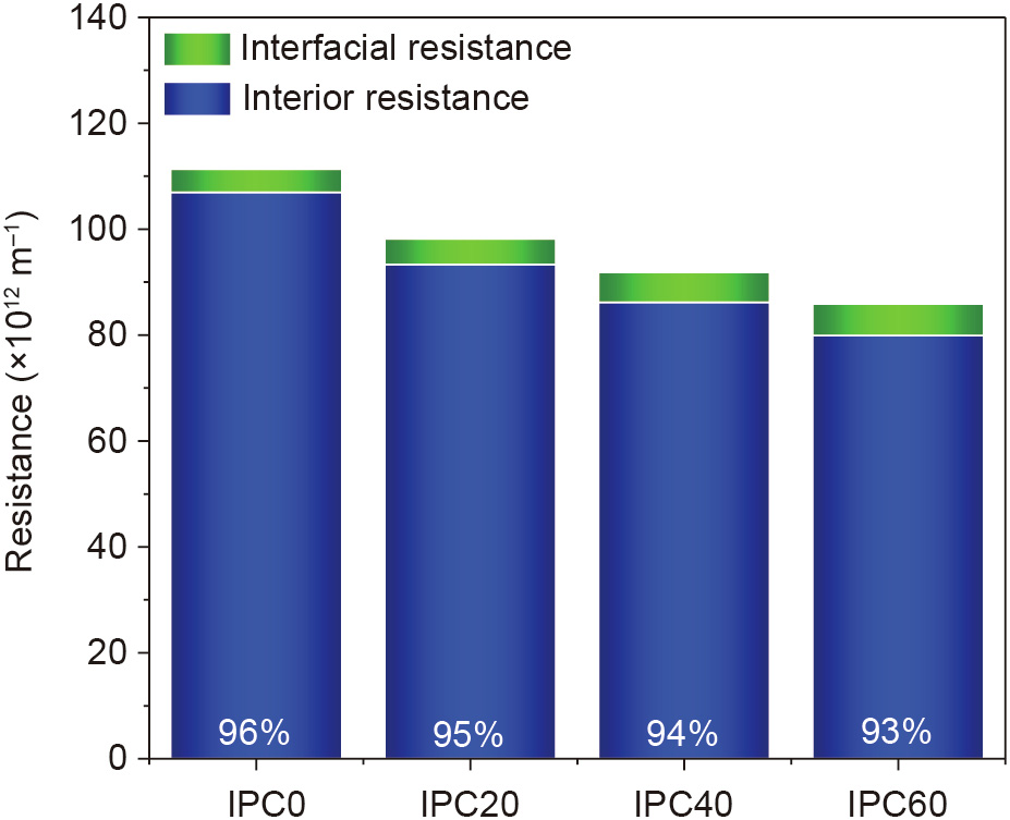
Fig. 7. Extrapolated resistances of the membranes (thickness = 200 nm) with various IPC contents.
According to this finding, the total resistance of RO membranes can be efficiently reduced by reducing the interior resistance of the PA layer. A common means to this end is to prepare a thinner PA layer—mainly by changing the parameters of the interfacial polymerization—that aligns with the experimental observations. However, because of the extremely fast process of interfacial polymerization, the thickness of the PA layers can only be reduced within a relatively limited range. Alternatively, in addition to tuning the thickness of the PA layer, the interior resistance can be efficiently reduced by modifying the chemical composition of the PA layer. This was done by extrapolating the PA layers with a constant thickness of 200 nm produced from mixed monomers with changing ratios. Fig. 7 also shows that the total resistance drops with increasing IPC contents, which implies that a larger water flux can be expected for membranes prepared from recipes with higher IPC contents. Impressively, such an understanding is in excellent agreement with the experimental results [16].
Recently, Zhao et al. [16] carried out an interesting work to investigate the effect of the chemical composition of the PA layers on RO performance by using a mixture of two acyl halide monomers, BTEC and IPC, to react with MPD in the interfacial polymerization of PA. They found that there was a constant increase in water flux with increasing IPC content, at no sacrifice of ion rejection. For example, the water flux increased by 34% when the IPC content increased from 0% to 60%. In order to have a direct comparison with these experimental results, we listed the estimated water flux of membranes with a 200 nm PA separation layer under a pressure drop of 5.5 MPa in Table 2. It is clear that the water flux is enhanced with increasing IPC contents. At the same time, no ion was observed to pass through the membranes, and no ion could even permeate into the PA region. Consequently, 100% ion rejection was obtained for all the cases. Moreover, the water flux increased from 48 to 63 L·m-2 h-1 when the IPC content increased from 0% to 60%. That is, the water flux was enhanced by 31.25%, which is in excellent agreement with the experimental results [16]—not only in terms of the trend, but also in terms of the enhancement in pure water flux.
《Table 2》
Table 2 Estimated pure water flux under experimental conditions (5.5 MPa, 200 nm thickness) and ion rejection of the membranes with various IPC contents.

《4. Conclusions》
4. Conclusions
In this work, we investigated the transport resistance of water in PA RO membranes by separately considering the interfacial resistance and the interior resistance. The models for these two contributions to the transport resistance were built with and without water reservoirs, respectively. The interior resistance is dependent on the thickness as well as on the chemistry of the PA layer. When the thickness is small, for example, at 5 nm, which is the typical length scale for simulations, the interior resistance plays a minor role while the interfacial resistance contributes more than 62% of the total resistance. Importantly, we found that the two contributions should not be proportionally multiplied for thicker PA layers because the interfacial resistance is independent of the thickness of the PA layers. Since PA layers for real-world RO membranes typically have a thickness of 200 nm, the interfacial contribution decreases significantly to less than 10%. To investigate the effect of the chemistry of the PA layers on the two resistances, we investigated RO membranes that were prepared from the interfacial polymerization of a mixture of two acyl halides with MPD. The interior resistance dropped while the interfacial resistance increased with a decreasing number of residual carboxyl groups in the PA layers. However, as the interior resistance plays the dominant role, the total resistance decreased with a decreasing number of residual carboxyl groups. These findings are in excellent agreement with the experimental results in terms of both the trend and the flux enhancement. These simulation findings increase our understanding of water transport in RO membranes, allowing reliable prediction of water flux on the one hand, and guiding the rational design of high-flux RO membranes on the other.
《Acknowledgements》
Acknowledgements
Financial support from the National Key Research and Development Program of China (2017YFC0403902), the National Basic Research Program of China (2015CB655301), the National Natural Science Foundation of China (21825803), the Jiangsu Natural Science Foundations (BK20190085 and BK20150063), the Program of Excellent Innovation Teams of Jiangsu Higher Education Institutions, and the Project of Priority Academic Program Development of Jiangsu Higher Education Institutions is gratefully acknowledged. We are also grateful to the High Performance Computing Center of Nanjing Tech University and the National Supercomputing Center in Wuxi for supporting us with computational resources.
《Compliance with ethics guidelines》
Compliance with ethics guidelines
Yang Song, Mingjie Wei, Fang Xu, and Yong Wang declare that they have no conflict of interest or financial conflicts to disclose.
《Appendix A. Supplementary data》
Appendix A. Supplementary data
Supplementary data to this article can be found online at https://doi.org/10.1016/j.eng.2020.03.008.


 京公网安备 11010502051620号


