《1. Introduction 》

1. Introduction

In microfluidic channels, the flow is usually in the lowReynolds-number laminar state due to the small dimension and the often highly viscous working fluids. The Reynolds number, Re , where U is the mean velocity of the channel flow, L is the channel hydraulic diameter, and v is the kinematic viscosity, represents the relative significance of the inertial force and viscous force. Unlike multiphase flow, which tends to form dispersed flow structures [1,2], single-phase flow maintains a consistent crosssectional distribution throughout a regular-shaped channel without external interference [3]. To realize specific lab-on-a-chip functions, such as biomolecular analysis [4], high-throughput screening [5], and chemical reaction control [6–8], which require the microflow to change the distribution, several flow engineering methods have been developed. Some methods intentionally increase the flow instability to achieve turbulent mixing, while leaving the flow profile unregulated [9]. Although active electrical [10] and magnetic [11] approaches have been extensively studied for highperformance flow rearrangement, these methods require complicated theoretical analysis to achieve delicate control. Furthermore, the dedicated equipment required and the complicated system setups prevent these methods from wide application. In comparison, some passive methods alter the flow distributions by introducing transversal secondary flow with specially engineered channel geometries, such as herringbone grooves [12], expansion chambers [13], or spherical obstacles [14]. Through the integration of these channel substructures, hydrodynamic flow focusing [15–17], fabrication of three-dimensional (3D)-shaped microparticles and microfibers [18–20], and custom hydrophoresis for particle focusing and sorting [21,22] can be realized. Despite the successful applications of engineering flow profiles, the flow profiles usually result from repeating simple secondary flow patterns. Moreover, due to the specific correlation between the structures and the flow field, the existing channels can hardly be generalized to produce profiles with different shapes. Consequently, a channel design for producing new types of flow profiles requires recursive trials and corrections, constraining the efficiency of new profile design. Therefore, a systematic method to engineer flow profiles is highly demanded.

To address this demand, hydrodynamic focusing with configurable microstructures has been introduced to produce a variety of complex flow patterns [23,24]. These methods deploy recessed strips or micropillars inside the microfluidic channel to focus and shape the flow. By modifying the transversal position and the dimensions of the posts, the range and direction of flow movements can be readily tuned, thus allowing customized modifications of the flow profile [14]. Moreover, these methods use selfprogrammed software to design and predict the final output profiles [24]. With the development of optimization algorithms, reverse design of the microstructure sequence from a targeted output flow profile can also be achieved [25]. These methods enable a wide variety of applications, ranging from the fabrication of particles and fibers with 3D cross-sectional shapes [23,26] to cell focusing and encapsulation [27]. Despite the remarkable performance, in most previous flow engineering methods, the working fluids operate in the inertia regime, where specific profile modifications require the precise replication of both fluid properties (e.g., viscosity) and flow conditions (e.g., Reynolds number), since the inertial flow is very sensitive to flow conditions [28]. Consequently, the produced profiles are vulnerable to velocity fluctuations, and previously designed profiles for a specific flow environment are inapplicable under different flow environments. Moreover, the geometry of the microstructures not only induces inertial behaviors of the flow, but also inherently rearranges the streams in regions with changing geometry. The coupling of these two effects complicates the correlation between secondary flow movement and microstructure geometry. As a result, a change in the microstructure geometry may cause unexpected secondary flow variations, with no clear guiding principles available for designing the microstructures. Unlike that in inertial flows, the inertial force in a Stokes flow is insignificant when compared with the viscous force originating from the channel geometry boundary. Although inertial behavior is intrinsic to any fluid flow, it is negligible in microfluidic environments, viscous aqueous two-phase systems [26], and polymer fluids where the Reynolds number is relatively low (< 1). Thus, the insensitivity of a Stokes flow to changes in the flow environment facilitates microfluidic flow-profile engineering.

In this work, we report a systematic method for engineering the flow profile in the Stokes flow regime, which we referred to as ‘‘inertialess flow shaping.” Sequenced steps are used as flow operation elements in microfluidic channels in order to investigate their flow redistribution effects. To speed up the flow-profile design, we develop a program to predict flow profiles by tracing the streams passing through discretized profile regions, where the predicted profiles agree well with the experimental observations. Based on the developed tools, we further demonstrate that our method enables the generation of an extensive variety of flow profiles. Compared with conventional methods, this method can generate flow profiles that are insensitive to flow fluctuations, and the channels can be easily adapted for a wide range of flow conditions with different fluids and flow rates.

《2. Methodology 》

2. Methodology

《2.1. Numerical study of flow redistribution around each microstep》

2.1. Numerical study of flow redistribution around each microstep

In this study, microsteps were placed in pairs on the top and bottom walls of the channel. The flow redistribution for a variety of steps was verified by examining the streamlines of the flow and the simulated flow profiles in the inlets and outlets. To visualize the flow redistribution around a single step, the trajectories of massless particles in the flow were tracked and drawn on the crosssectional planes upstream and downstream of the steps. The flow in the channel was considered to be a single-phase laminar flow and was simplified based on the following assumptions: As the flow was in the Stokes regime, the mass and momentum conservation equations of the system were solved without introducing any turbulence models. The ambient temperatures were assumed to be constant and homogeneous throughout the channel, such that heat transfer was avoided. The channel walls were assumed to be rigid and impermeable. The inlet conditions were defined by the inflow rates consistent with the experimental settings, while the outlet conditions were defined as the atmospheric pressure level. The computational fluid dynamics (CFD) case was computed using the commercial software Fluent (ANSYS Inc., USA).

《2.2. Programmed flow-profile prediction of predefined steps》

2.2. Programmed flow-profile prediction of predefined steps

The program transformed the inlet flow profiles to the outlet flow profiles by transforming each discretized flow parcel in the inlet flow profile to the corresponding position in the outlet profile. The displacement of each flow parcel was determined based on the pathlines calculated from the CFD simulations. First, the inlet flow profile was discretized into ‘‘pixels.” The area of each pixel was allocated to be inversely proportional to the area integration of the flow velocity, resulting in an equivalent fluid volume passing through each pixel. Second, the pixel coordination was established according to the row/column position of the pixels. The solute concentration or fluorescence intensity was assumed to be homogeneous within each pixel of the flow profile, and was represented by a value. Therefore, the flow profiles could be represented as a two-dimensional (2D) array. Third, to acquire the mapping relation between the inlet and outlet flow profiles around each step, the streamlines between the inlet and outlet of each microstep were simulated using CFD. The cross-section coordinates of the head and tail of each streamline, corresponding to the inlet and the outlet, respectively, were extracted and transformed into the pixel coordinates to form the pixel mapping models. During the profile transformation, the elements of the inlet flow-profile array were rearranged according to the pixel mapping models to construct the outlet flow profile. In the case of multiple streamlines starting from the same pixel, the value of the pixel was equivalently divided and assigned to each streamline. The profiletransformation function only needed to be calculated once and was then saved in a profile function library for future use. For channels with multiple steps, the outlet flow profile was calculated by superposing the flow transformation functions of the steps sequentially onto the inlet flow profile. Finally, the cross-sectional outlet flow profile was reconstructed by drawing each pixel area with the flow intensity, while the top-view flow profile was computed and visualized by summing all the area-integrated pixel values of the cross-sectional profile along the z-direction. The program was written in Python 3.7 with the packages NumPy 1.18.1, SciPy 1.4.1, Pandas 1.0.1, and Pycairo 1.19.1.

《2.3. Microfabrication of the structured channel》

2.3. Microfabrication of the structured channel

To ensure that the flow behavior around each microstep was independent of the adjacent microsteps, a sufficiently large distance between the inlet channel joint and each microstructure was provided to ensure fully developed flow before and after the flow redistribution range around each microstep. For better alignment of the two poly(dimethylsiloxane) (PDMS) slabs, triangular and rectangular structures were added to each of the slabs for precise matching of the spatial position. These matching markers were distributed alongside the channel of the chip’s boundary to enhance the precision of the fabricated chip, particularly in the areas where the fine features were embedded (Fig. S1 in Appendix A). The channels with microsteps on both the top and bottom walls were divided into two parts along the horizontal center plane and fabricated separately. Each part contained a single layer of microstructures (Appendix A Fig. S2). The PDMS slab containing each channel part was fabricated with high precision using the conventional technique of lithography replica molding: First, the molds were fabricated by lithographic patterning the SU-8 photoresist (SU-8 2075, Kakayu Advanced Materials, USA), which was spin-coated onto a silicon wafer (N100, UniversityWafer, USA). Subsequently, the channels were cast with PDMS (Sylgard 184, Dow Corning, USA) on the molds and baked at 65 °C for 6 h to achieve a high rigidity. After being peeled off, the PDMS slab of the bottom layer was first bonded to a glass slide (ISOLAB, Germany) after being charged with a plasma cleaning machine (PDC-002, Harrick, USA), and then bonded to the top layer. By further baking at 95 °C, the bonding between the charged surfaces was strengthened. Before every experiment, the channel walls were made hydrophilic by injecting ethanol into the channel to prevent air bubble entrapment at the sharp corners of the microstructures.

《2.4. Experimental verification of the designed flow profile》

2.4. Experimental verification of the designed flow profile

To verify the customized flow profiles, we used a mixture of 80% glycerol (Sigma-Aldrich, USA) and 20% deionized water, which was highly viscous, to guarantee Stokes flows. To visualize the flow profiles of different streams in the single phase, fluorescein was used to stain the target streams at a concentration of 2 mg·L^-1 . Syringe pumps (neMESYS 290N, CETONI, Germany) were used to introduce the dyed fluids and transparent fluids into the channel to form vertical color bands. The flow profile width and position were adjusted by modifying the relative flow rate of the inlets. When the flow reached a steady state, the top-view flow pattern was captured by means of a fluorescence microscope (Leica Camera, Germany), and the cross-sectional flow profile was acquired using a confocal microscope (LSM 710 NLO, ZEISS, Germany) and imageprocessing software (ZEN2010 Black Edition, ZEISS, Germany).

《3. Results and discussion 》

3. Results and discussion

《3.1. Performance and feasibility of inertialess flow-shaping schemes》

3.1. Performance and feasibility of inertialess flow-shaping schemes

We deployed geometric microsteps inside rectangular microchannels to induce flow deformations. As the ‘‘inertialess” fluid flows through the steps, its original spatial arrangement is disturbed due to the geometric changes, resulting in a deformed flow profile. Each microstep is considered to be an element flow operator and to induce a unique profile distortion, depending on the geometry. By introducing steps with various geometries in sequence, we generated a broad range of complex flow profiles (Fig. 1). The concept of using sequenced microstructures to engineer flow profiles is similar to previously developed methods [24,29] that use the inertial behavior of the flow to generate transversal secondary flow, but that only work at relatively high Reynolds numbers (> 5). Furthermore, the inertial behavior of the flow is highly sensitive to the velocities and boundary geometries. Therefore, in order to engineer a predefined working fluid to obtain the desired profile, the required flow conditions must be unique and stable.

《Fig. 1》

Fig. 1. An overview of the inertialess flow-shaping method. Microsteps are alternately deployed on the top and bottom walls. The flow profile of the target stream is progressively shaped by the sequenced microsteps. The images in red boxes above the channel schematics show the top views of the flow distribution around each crosssection indicated by the orange borderline shown in the channel schematic. The first, second, and fourth steps are asymmetric chevron-shaped steps with an oblique angle of 60° on both sides, and the third step forms a 60° angle to the channel axial direction. The bottom row of images illustrates the flow profiles at each cross-section (scale bar: 50 μm).

The Stokes flow has not been sufficiently considered for profile engineering, as its inertia-free behavior prevents irreversible changes of the flow profile after the flow parcel passes through simple obstacles, such as pillars and spheres [14,24]. Therefore, engineering a Stokes flow requires more sophisticated structures. To simulate the conditions for flow deformation to occur in the Stokes flow regime, we numerically calculated the flow distributions around a set of steps with different shapes (Fig. 2(a)). Two stages of profile deformation were observed: First, the original rectangular flow profile is nonlinearly compressed to the crosssectional shape at the upstream facet of the step, with the change in step geometry deflecting the local flow toward the normal direction of the step faces. Second, the compressed flow profile is restored to a rectangular shape, while the step-proximal secondary flow deflects toward the opposite normal direction of the downstream step facets (Fig. 2(b)). To reclaim the original flow profile, all displaced flow parcels must return to the original crosssectional positions. The fore–aft symmetric steps ensure that the flow parcel will move along a reversed path to its original position, while the laterally symmetric steps ensure that the flow parcels in all directions will have equivalent displacements. Hence, the steps need to be fore–aft or laterally symmetric in order to maintain consistent flow profiles before and after the flow parcel passes the steps. Steps without geometric symmetry in the axial or lateral direction would cause unbalanced profile compression and expansion, inducing a net flow-profile deformation.

《Fig. 2》

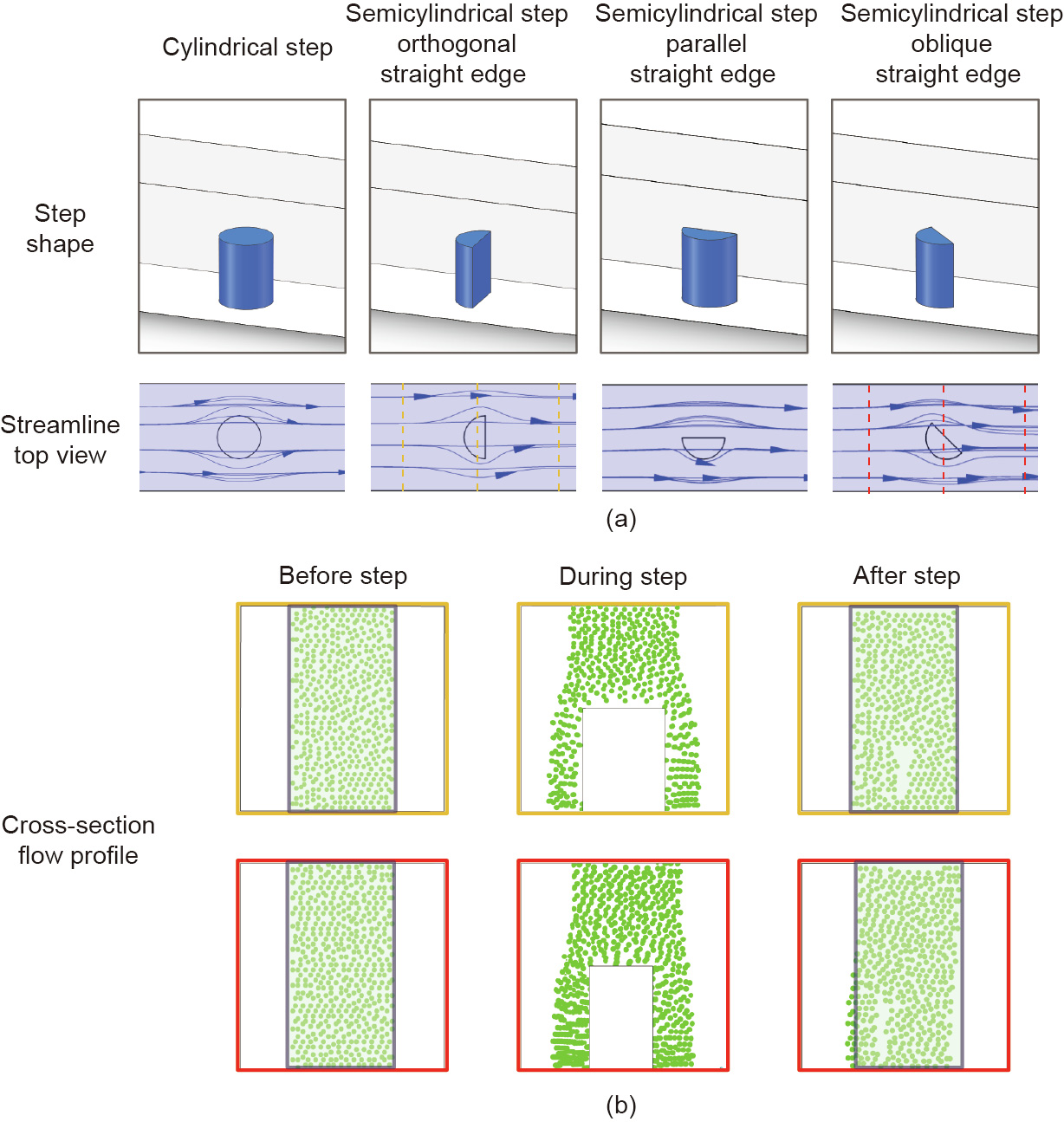
Fig. 2. Deformation of the flow profile by different microsteps in the Stokes flow regime. (a) The flow distribution around (left) a cylindrical step, (center) semicylindrical steps with the straight edge orthogonal and parallel to the channel axial directions, respectively, and (right) a semicylindrical step with an oblique straight edge; (b) the flow profile before, during, and after the step (the yellow and red border flow profiles correspond to the cross-sections denoted in yellow and red in the top views; the profiles are assembled from the streamline intersecting positions in the cross-sections of the channel).

Unlike the inertial flow, which is sensitive to the flow conditions, the Stokes flow behavior is less dependent on the flow conditions. We numerically investigated the stream distributions around the steps under different flow rates. For each step, the output flow profiles are invariant when the Reynolds numbers are below one, regardless of the scales of the channel or the net flow rates (Fig. 3(a)). The profiles for the cases of Re = 5 and Re = 10 show inconsistent flow deformation, indicating the presence of inertial flow. As a result, the present method only works for a Reynolds number less than one, where the effect of the inertial force is negligible, and the geometry of the steps determines the flow rearrangements. Hence, once the structure of the step is determined, the channel is expected to induce consistent secondary flow for a wide range of flow conditions in the Stokes flow regime.

The flow redistribution effect of the steps can be adjusted by tuning the geometry, scale, and position of the steps. To reduce the parameters in the step design, we used quadrangular prisms as the elemental steps, with the side edges parallel to the channel axial direction and the upstream and downstream edges oblique to the channel axis. All the steps were regulated to have uniform heights. This framework of the step ensures that only the upstream and downstream facets will be configured for tuning the flow deformation. By adjusting the axial angle of the upstream and downstream edges, various local flow-profile deformations can be achieved. Moreover, the elemental steps can join in parallel to form a combined-shape step, thereby realizing versatile flow deformation direction and amplitude. Since the steps can only deform the proximal flow profile, the size and lateral position of the step can also be customized to tune the degree and range of the local profile deformation.

The steps of various configurations can be placed sequentially inside a channel to produce more complicated flow profiles. The distance between the adjacent microsteps is set sufficiently large for the flow to become fully developed, so that each step produces independent profile transformations. Since each step transforms the flow profile nonlinearly, the sequence of the steps also affects the output flow profile. Due to the unlimited step configurations and the logarithmically increasing possible sequences, the theoretical number of producible output flow profiles generated using this method is infinite. However, the profiles near the opposite wall of the steps can hardly be engineered because the step/channel height ratio is usually kept below 0.5, while the steps with larger height ratios significantly squeeze the cross-section of the flows and may induce inertial behaviors of the flow. Thus, deploying all the steps on a single wall fails to produce a fully engineered flow profile. In contrast, deploying the steps in pairs on two opposite walls can not only generate global secondary flow, but also change the flow profiles through the various combinations of the top and bottom walls (Fig. 3(b)). However, this type of channel design requires complicated fabrication equipment and processes, such as micro-machining [29], which are difficult to achieve using single-layer PDMS-based microfabrication. To address this problem, we placed the steps alternately on two opposite walls, with a height ratio of 0.5. As a result, the channel structure could be divided into two patterned PDMS layers, while the two PDMS layers could be manually aligned and bonded under an optical microscope by researchers without specialized training. The combination of numerical simulation and device fabrication removes the demand for high complexity in the fabrication procedures, thus speeding up the design and prototyping of channels for complicated flow profiles. Although the steps are arranged individually, the steps exhibit comparable performance to that of the paired steps and can still synergistically deform the flow (Fig. 3(c)).

《Fig. 3》

Fig. 3. Secondary flow patterns generated from different step configurations. (a) Output profiles of a single step at various values of the Reynolds number; (b) comparison of the flow deformation effect of single steps and paired steps (the dot cloud denotes the passing-through positions of streamlines coming from different inlets, and the arrows show the trends of the transversal flow); (c) comparison of the flow-profile deformation between paired steps and alternately arranged steps (the orange and green profiles in the bottom right figures are numerically predicted based on the alternate microstructure channel and the paired microstructure channel, respectively).

《3.2. Program-based flow-profile prediction and verification》

3.2. Program-based flow-profile prediction and verification

Although CFD methods enable accurate prediction of the flow profiles around a single step, the simulation of a channel with multiple steps is impractical due to the overwhelming amount of mesh required for a satisfactory total error level. Moreover, for every new structured channel, a new simulation case is needed, which significantly limits the speed of channel structure design. To efficiently predict the output profile of a sequence of predefined steps, previous methods convert the employed steps into independent transformation functions and superpose the functions onto the step sequence [25,30]. Employing this logic, we have developed a compact profile-discretization-based algorithm to realize the superposition of flow-profile transformations, as illustrated in Section 2. The accuracy of the CFD simulation is ensured by deriving converged and mesh-independent results (Fig. 4). Despite the local information loss, the computed top view of the flow distribution matches well with the experiment results, even for multiple steps (Fig. 4(a)).

Based on the previously described procedures, flow-profile transformation functions are built from the computed streamline information. To obtain solid profiles without elevating the numerical prediction error, balanced ceiling and floor thresholds of the filter are applied. Taking widthwise strip-shape steps as an example, using the current simulation and prediction algorithm settings, the predicted top-view flow distribution and flow profile agree with the experimental results for more than 15 microstructures (Fig. 4(c)). Moreover, the flow profiles under various flow rates are demonstrated to be stable as the flow rates range from 400 μL·h^-1 (Re ≈ 9.6 × 10^-4 ) to 3200 μL·h^-1 (Re ≈ 7.7 × 10^-3 ), which suggests that the program can accommodate a wide range of flow conditions without further modifications (Fig. 4(d)). For Re > 1, the present method can also output flow profiles similar to those produced at Re < 1, with minor nonlinear distortions resulting from the inertial secondary flow. This distortion of profiles will intensify with increasing Re and the number of steps involved in generating secondary flow. Therefore, to ensure high consistency of the flow profile of various flow rates and flow motions, we propose to engineer the flow profile in the Stokes flow regime. Despite the requirement of a low Reynolds number, the flow rate can still reach the scale of several milliliters per second for fluids with high viscosity, which is the case for many microfluidic applications (Fig. 4(e)). However, the current program has a limitation: The values of some of the profile pixel tends to dissipate during weighted streamline transportation. Consequently, as the number of microstructures increases, pixel intensity fading becomes inevitable across the whole profile (Fig. 4(b)). This systematic error can be further attenuated by narrowing the filter passband. Furthermore, during the prediction of the profiles after multiple microstructures, the loss of profile pixels is amplified during the iteration of the transformation functions. This issue arises from the CFD results and limits the maximum number of reliably predicted microstructures.

《Fig. 4》

Fig. 4. (a) Comparison between the CFD-simulated streamline distribution and the experimental observations after five repeated 60° oblique steps (#5) and three reapeated 30° oblique steps (#3), respectively (scale bar: 100 μm). (b) predicted profile after 20 iterative transformations and the derived top view matches the experimental result well; the predicted profiles after 5, 10, 20 steps are denoted with #5, #10, #20, respectively. (c) Predicted flow profiles and experimental profiles after 15 steps (scale bar: 50 μm). (d) Experimental flow profiles produced using the same channel under the specified flow rates (Q). The experimental profile images are the orthogonal images of the z-stack images captured with a confocal microscope. The experimental top-view images in parts A and B in Fig. S1 are captured with a fluorescence microscope, and the experimental profile images are the orthogonal images of the z-stack images captured with a confocal microscope (scale bar: 50 μm). (e) Phase diagram depicting the profiles at different viscosities and flow rates (the blue region is the inertialess flow-shaping range, while the yellow region is the inertial profile-engineering range; the phase line is drawn at Re = 1, where noticeable inertial secondary flow starts to arise; and the profiles are produced in the same channel based on their local viscosity and flow rates).

《3.3. Inertialess flow shaping of alternate side microsteps》

3.3. Inertialess flow shaping of alternate side microsteps

With the flow-profile prediction program, it was possible to efficiently investigate the profile-shaping capability of alternately sided microsteps. In our preliminary test, the transformation functions of four single-fold microsteps were produced. By applying these transformation functions in four different sequences to the same inlet flow profile, four different hydrodynamically focused flow profiles were obtained, with various delicate feature combinations. The delicate features, such as the hooks in Fig. 5(a), can be specifically engineered with other microstructures to perform different target functions according to the user’s needs. Moreover, non-intuitive flow transformation can be achieved by increasing the number and diversity of the microstructures. The channel design for a specific transformation, such as hydrofocusing and profile rotation, can be recorded as standard design elements and can directly contribute to a broader range of profile formations. By further increasing the number of input profile bands, composite flow profiles with different division morphologies can be obtained. This inlet setup was realized in the experiments by increasing the number of inlets, with different reagents being fed into different inlets to form compound profiles (Fig. 5(b)). In general, to produce a flow profile, a generalized strategy should start with hydrofocusing the target flows away from the walls, followed by shaping the overall shape by global simple-shape steps and sculpting the delicate features with locally engineered steps.

Compared with previous inertia-based profile-engineering methods, the current method avoids a reliance on the flow inertial behavior, and thus facilitates profile shaping in low-Reynoldsnumber applications. Inertia-based methods use pillars [24] or top–down symmetric structures [29,31] to transform the flow profile, which can hardly produce asymmetric flow profiles [23,24,29]. In contrast, the geometric symmetry of the steps used in the current method can be freely configured, without increasing the design complexity. Hence, the present method can be extended to the design of asymmetric profiles.

《Fig. 5》

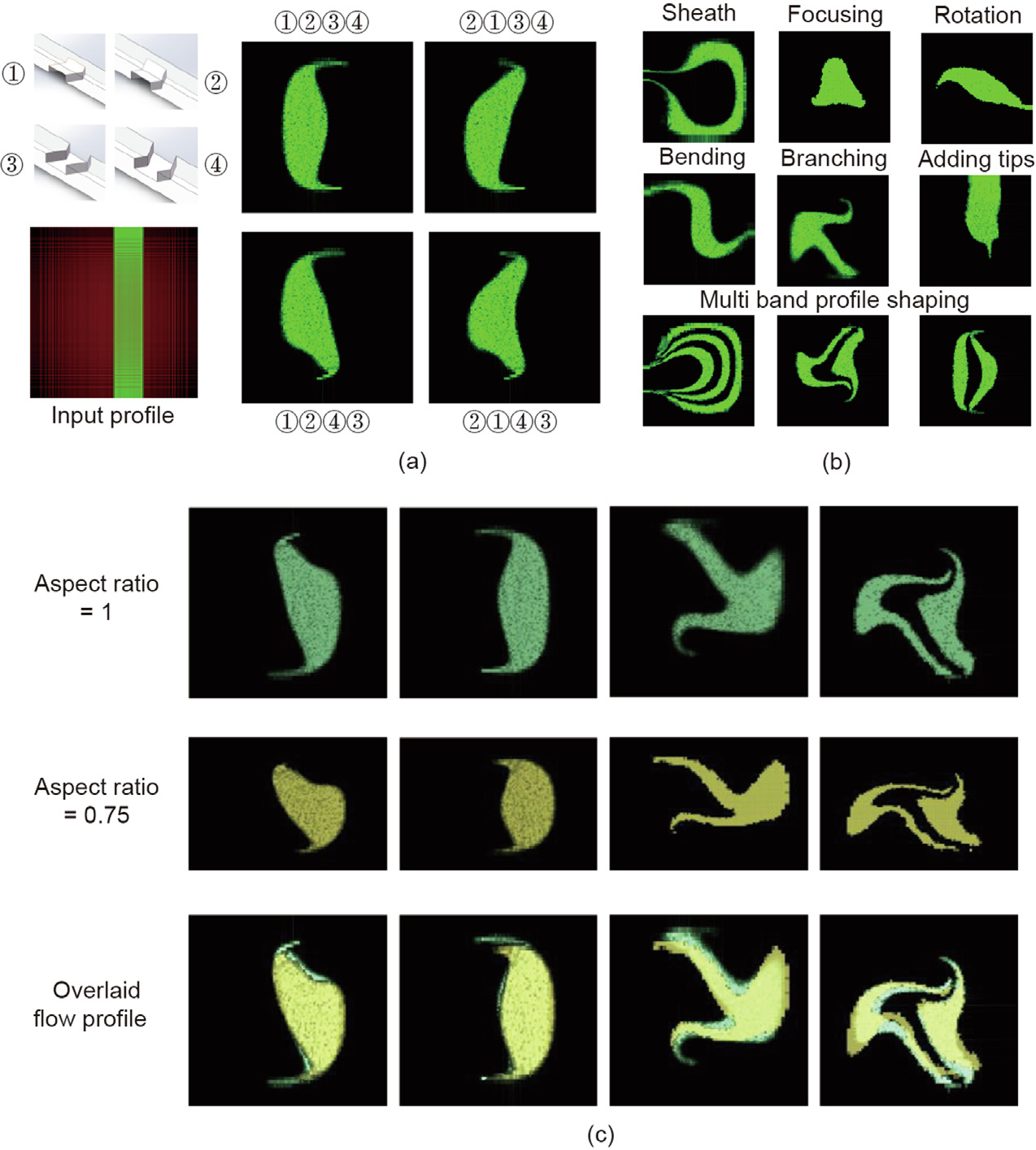
Fig. 5. Profiles designed and predicted using the custom program. (a) Using the same set of steps, the small features can be customized (steps ① and ③ are eccentric chevronshaped steps with a 60° oblique angle on each wing, while steps ② and ④ are mirrored along the channel axial line from steps ① and ③); (b) examples of achieved profile shapes (the steps employed and the step sequence required for each profile are listed in Appendix A Tables S1 and S2); (c) variations in the flow profile for channel aspect ratios of 1 and 0.75.

For a profile-engineering method to be universal, the flow profile must be reproducible with a wide range of flow conditions. In conventional flow engineering methods, the flow-profile deformation depends on the substructure geometry and the inertial property of the fluid, as well as the flow velocities. Consequently, the flow profiles are bounded to the specific sets of flow conditions used in the design process. A change in the working fluids or flow condition fluctuation could cause significant profile distortion [23], making it difficult to reproduce the flow profile designed using conventional methods with another fluid material or under different flow conditions for the same channel settings. In contrast, the flow distribution of the inertialess flow only depends on the geometry of the channel, which demonstrates that the flow profile can be reproduced with any fluid viscosity or flow rates, as long as the Stokes flow condition is satisfied (Table 1). In our experiments, the observed flow profiles remain consistent even when the flow rate is magnified by eight-fold (Fig. 4(d)), and the normalized flow profiles are insensitive to changes in the channel aspect ratios. Thus, a similar profile can be achieved in channels with different aspect ratios (Fig. 5(c)). Since only the channel geometries need to be considered, the reduced dependence on the flow conditions and channel geometry can significantly simplify the flow-profile design process. Moreover, the predesigned flow profiles and the corresponding channel structures can be recycled for various works without the need for case-specific adjustments. Despite the advantages of inertialess flow shaping, the present method has limitations. In the simulation, the channel walls are assumed to have no-slip boundary conditions, but physically, the slip flow exists. In principle, the wettability of the wall influences the slip flow and thus affects the flow distribution in the channel [32]. From our experiments, we found no major differences between the predicted flow profile and the experimental profile, indicating that the step wettability has only a minor influence on the flow profile. However, vast changes in wettability, such as when using a glycerol solution or silicone oil, could cause noticeable profile variations (Appendix A Fig. S3). Therefore, the inertialess flow-shaping method is more suitable for aqueous solutions in a PDMS channel. Moreover, the present method works at a flow rate only one to two magnitudes lower than the conventional inertial flow-based methods, limiting the rate of production of fibers or particles.

《Table 1》

Table 1 Comparison of the inertialess flow shaping and inertia-based flow engineering methods.

《4. Conclusions》

4. Conclusions

In this work, we presented a universal flow-profile engineering method operating in the Stokes flow regime using microsteps. By tuning the geometry, size, and lateral position of the steps, we were able to customize the flow-profile deformation. Complex flow profiles could be generated by sequentially arranging various steps inside a channel. Moreover, a prediction program was developed to predict the flow profile based on discretized profile-shaping regions, with excellent agreement between the profile predictions and the experimental observations. Compared with conventional flow-profile engineering methods, the inertialess flow-shaping method can achieve a wider range of possible profiles. Operation in the Stokes flow regime enables a simplified profile design, which can be conveniently generalized to a wide range of flow conditions and fluid materials. The new method offers practical guidance for engineering flow profiles in flows with a Reynolds number below one, thus facilitating applications such as fabricating specially shaped microfibers and microparticles.

《Acknowledgements 》

Acknowledgements

This work was supported by the General Research Fund (17306315, 17304017, and 17305518) and Research Impact Fund (R7072-18) from the Research Grants Council (RGC) of Hong Kong, China, the Excellent Young Scientists Fund (Hong Kong and Macau) (21922816) from the National Natural Science Foundation of China (NSFC), the Seed Funding for Strategic Interdisciplinary Research Scheme 2017/18 from the University of Hong Kong, as well as the Sichuan Science and Technology Program (2018JZ0026).

《Compliance with ethics guidelines 》

Compliance with ethics guidelines

Zhenyu Yang, Lang Nan, and Ho Cheung Shum declare that they have no conflict of interest or financial conflicts to disclose.

《Appendix A. Supplementary data 》

Appendix A. Supplementary data

Supplementary data to this article can be found online at https://doi.org/10.1016/j.eng.2021.02.008.