

《1. Introduction》
1. Introduction
The electronic band structure plays a fundamental role in our understanding of the origins of the physical properties of materials and in assessing paths for optimization and chemical substitutions. The dispersion relation of the solutions of the many-body electronic Schrödinger equation provides quantitative information that is essential for understanding most of the functionalities that a material may exhibit. The band structure,  , is a mapping from
  (where N is the number of relevant bands, n the band index, and k a vector indicating the crystalline momentum) and is usually represented by considering only two-dimensional (2D) band plots. Because any given band is a function whose domain is the three-dimensional (3D) Brillouin zone (BZ),
  , the graph of a given band is embedded in four dimensions. Band structure plots along high-symmetry lines are a useful tool for evaluating a material at a glance. However, the 2D representation hides the full complexity of the electronic spectrum by ignoring large sections of the BZ. Conventions, such as those in Ref. [1], provide common ground for band plots, but 2D band representations are intrinsically limited.
Critical points, where  = 0 (with
  indicating the gradient of with respect to k), are an important feature of the electronic band structure. At these points, the density of states (DOS; also represented by the function of energy E, D (E)) is large (or diverges; see Ref. [2])
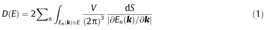
with the unit cell volume V and an infinitesimal element of the constant energy surface dS. Critical points are key in evaluating a material’s physical properties and fully characterizing the material. For example, for a 2D material, it is well known that saddle points lead to logarithmic singularities [3], and that maxima and minima in three dimensions lead to square root dependencies of the DOS and, in general, to van Hove singularities or non-smooth points [4]. Thus, the identification of all critical points is an important goal.
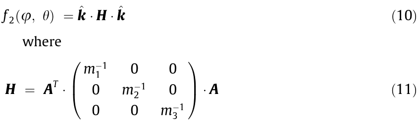
A related concept associated with the local properties of the electronic band structure involves the effective mass tensor M* , which is—assuming Taylor expansibility near k0—a second-rank tensor in 3D with components:

where n is the band index,  is the reduced Planck constant, me is the mass of electron, and the subscripts i, j are used to label the Cartesian components of the tensor M* or of the vector k. The reciprocal of the effective mass tensor is associated with the curvature of the energy dispersion, , and is a critical descriptor when discussing electronic transport and optical properties; its evaluation must be done by considering the full mathematical complexity of the band structure. In addition, the possible presence of non-analytic points—such as points where the Hessian is not a symmetric matrix—leads to warped critical points, which play a role in several situations [5,6] but are difficult to identify with 2D band plots. By determining high-fidelity effective mass tensors at critical points, it is possible to formulate analytic models of band structures. Such models are important in many considerations in solid-state physics and electronic engineering; for example, they can be used as a starting point for Monte Carlo transport simulations [7] or for the multi-scale modeling [8] of electronic devices, batteries, and thermoelectric energy converters. Analytic band structures are used in applications such as modeling scattering rates where derivatives and integrals of the bands are necessary [7]. From an experimental standpoint, the DOS effective mass is a common property of the band structure that may be measured through cyclotron resonance [9-18], the four coefficients method [19], Shubnikov–de Haas oscillations [16,20-23], magnetophonon resonance [15,16,24,25], time-of-flight drift velocity [7,26-29], optical transmission and reflection [30-32], and infrared reflection and Faraday rotation [33-35]. Being able to compare the different measurements of the effective mass obtained with those indirect methods and reconcile such results with electronic structure calculations is a major goal.
This paper introduces a two-layer high-throughput (HT) methodology with the aim of partially addressing the misalignement between theory and experiment in the current literature. The first layer is a conventional chemical substitution/structural variation (e.g., see Refs. [36-42]), and the second is a careful exploration of to identify the nature of the critical points and compute the effective mass tensors. The conventional HT considers an array of prototypical materials: III–V semiconductors, filled and unfilled skutterudites, as well as rock salt and layered chalcogenides. For each material, we search the full BZ for critical points and determine the effective mass at those points using several different methodologies for verification [43]. These methodologies also characterize the warping of bands and correctly compute the DOS effective mass at those warped points [6]. To our knowledge, this is the first HT calculation of effective masses in a large portion of the BZ.
In Section 2, we illustrate the details of the computations. Section 3 presents selected results (a large part of the data is included in Appendix A), and Section 4 discusses the impact of this work.
《2. Methods》
2. Methods
The prototypical materials selected for this work are as follows: III–V semiconductors (AlSb and AlP with the zincblende structure); rock salt (PbTe, GeTe, SnTe, PbS, GeS, SnS, PbSe, GeSe, and SnSe) and layered chalcogenides (Bi2Te3, Bi2Te2Se, Bi2Se2Te, Bi2Se3, Bi2Te2S, and Bi2Se2S); and pristine and fully filled cobalt antimonide (specifically CoSb3, CaCo4Sb12, and BaCo4Sb12). For each material, the workflow starts by generating a projected atomic orbital tight-binding (PAO-TB) Hamiltonian, which is exploited to interpolate the band structure efficiently and precisely [44]. We use Quantum Espresso (Quantum ESPRESSO Foundation, United Kingdom) [45,46] to calculate the electronic structure in the AFLOWπ HT computational framework [47].
The AFLOWπ’s workflow (Fig. 1) drives the calculation of the Hubbard U correction within the ACBN0 [48-51] scheme (see Tables S1, S4, S14, and S18 in Appendix A), optimizes the structure of the unit cell, and generates the PAO-TB Hamiltonian. The wavefunction and charge kinetic energy cutoffs were 150 and 600 Ry (1 Ry = 2.179872 × 10⁻¹⁸ J), respectively, and a Monkhorst–Pack k-point grid with a density of about 0.01 Å1 has been used. The choice of pseudopotentials was driven by a need to maximize the number of well-projected bands in the PAO-TB model; for this purpose, Perdew–Burke–Ernzerhof (PBE)-projector augmented wave (PAW) pseudopotentials generated from the PSlibrary [52] were modified to have an extended basis [44]. The computations included spin–orbit coupling. For comparison and testing of warping, calculations without spin–orbit were also performed. PAOFLOW (University of North Texas, USA) [53] was used to project the computationally expensive Hamiltonian from the plane wave basis into the more efficient PAO-TB basis. The PAO-TB Hamiltonian allows the exploitation of the Fourier interpolation to obtain a smooth version of the band structure. The full BZ was divided into a 12 × 12 × 12 grid, and each voxel was searched for an isoated critical point. It was assumed that a voxel would contain at most one critical point. We chose a 12 × 12 × 12 grid to strike a balance between accuracy and computational efficiency. The locations of the critical points in k-space were then compared using operations of the symmetry group to identify unique critical points. This was done for ease of computation and for uniformity in analysis, given different crystal structures.
《Fig. 1》

Fig. 1. The AFLOWπ workflow script used in this study. More details on AFLOWπ are available in Ref. [47].
In order to identify critical points, we identified k-points, where the band velocities  are very small.

Fig. 2 shows a typical case of a saddle point for SnTe. The three panels show the three components of the velocity υ. The electron group velocity was calculated via the PAO-TB Hamiltonian by taking the expectation value of the momentum operator p, as discussed in Ref. [2]

where me is the electron mass, H is the Hamiltonian, and ψn is the single-particle wavefunction.
《Fig. 2》
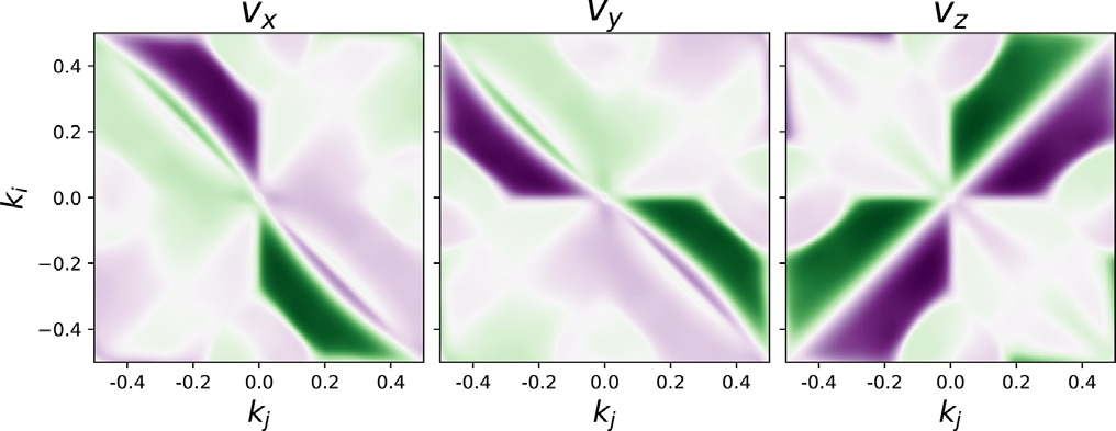
Fig. 2. A 2D slice k = ( i, j, 0.5) of the 3 components of the gradient of the energy for the bottom conduction band in the first BZ for SnTe. The purple and green represent k with large positive and negative values, respectively, for each gradient component.
Starting from the energy dispersion, we computed the Hessian matrix using second-order Fourier derivatives [54,55]:

The inverse of the Hessian matrix is proportional to the effective mass tensor in the chosen reference system. Diagonalization of M* leads to the three eigenvalues m1, m2, and m3. The DOS effective mass is calculated by taking the geometric mean of the three effective mass components, m1, m2, and m3:

It should be noted that, in the definition of  , only one among the possible equivalent k-points is considered. The validity of the Fourier approach (which is very efficient computationally) holds for all non-warped bands but fails in the case of warped bands where the Hessian is not symmetric. In order to treat all the critical points in the same way, we calculated the inverse effective mass surface (IEMS) and used it to determine the three diagonal components of the effective mass tensor, the DOS effective mass accounting for band warping effects [6], and the band warping parameter (w) [5].
The IEMS was generated by interpolating the energy dispersion using a radial grid centered on each critical point. For each critical point and each angular direction in the spherical grid (defined by φ, θ, we found the second derivative of the energy dispersion along the radial direction kr—that gives, the effective mass in a given radial direction (Fig. 3) near  . The band curvature
  gives the second-order coefficient,
  , in the radial one-dimensional (1D) Taylor expansion (in natural units):

《Fig. 3》

Fig. 3. Energy dispersion in several radial directions around the degenerate, warped C point k = ( 0, 0, 0) near the Fermi level (Efermi) in CaCo4Sb12. The lattice parameter is indicated with a.
This angular form is very general [5] and allows for the treatment of non-analytic (hence warped, non-Taylor series expandable) critical points in the band structure. Similarly to previous work [5,6], we opted to fit our radial energy dispersion to a polynomial function greater than order two in order to account for possible band non-parabolicity, which can be clearly seen in Fig. 3. In order to calculate the three components of the effective mass, the DOS effective mass for warped bands, and the warping parameter, we fitted the values of the IEMS at a given critical point. We chose an expansion in real spherical harmonics to be a general form for future analysis.

The basis of real spherical harmonics,  includes the Condon–Shortley phase [56]. For analytic critical points, the diagonal form of the inverse effective mass tensor,
  was found by aligning a set of orthogonal axes with the maximal values of the IEMS. Fitting the surface in these coordinates to the simplified form, as shown in Eq. (9), gives the effective masses directly [5,6].

The direction of the maximal values of the IEMS aligns with the principal axes of the ellipsoids of constant energy and corresponds to a coordinate system in which the inverse effective mass tensor is diagonal. In general, the IEMS near an analytic critical point is a quadratic form:
is the matrix of second partial derivatives of the energy dispersion and A is the Euler rotation matrix (see Eq. 4.46 in Ref. [57]). Here,

is the angular  unit vector. The matrix H may be diagonalized to find the diagonal values as well as the directions of the principal axes. Alternatively, if the principal axes can be found first, as described above, the masses may be read off from a fit to Eq. (9). The algorithm is described as follows: Given the standard Cartesian basis X, Y, and Z defined by the coordinate system of the YlmS, let X' , Y' , and Z' be the axes after step ①, as defined below, and X'', Y'', and Z'' be the axes transformed from X' , Y' , and Z' with the transformation in ② below. The procedure can be done by ① finding Euler angles
  that rotates the reference Z axis to the direction of the maximum absolute value of the IEMS; and ② with a fixed from the previous step, rotating the X' axis around the Z' axis until it achieves a maximum value. The third direction is orthogonal tothe Z'' = Z' and X'' axes in a righthanded coordinate system. The value of the IEMS along the X'', Y'', and Z'' axes corresponds to
  , respectively. In the case of non-analytic critical points, the DOS effective mass
  is computed by integrating a particular function of the IEMS [6] over the entire angular surface at a given point:

The sign of the integral depends on the sign of the IEMS. For saddle points, the value of the integrand in Eq. (14) approaches infinity when  approaches zero. In principle, one can integrate over the range of φ and θ where is positive and separately where it is negative. In practice, however, it proves difficult to achieve convergence for the integral, and we do not include the calculation of the DOS effective mass for warped saddle points in our results. To the best of our knowledge, the problem of properly accounting for saddle points is still unsolved.
《3. Results》
3. Results
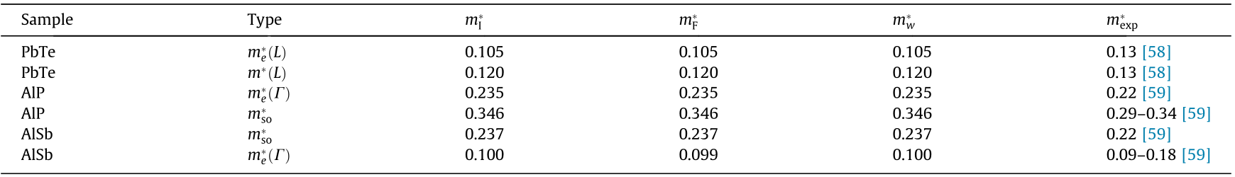
There is a wide range of effects on the DOS and other material properties from the local band structure at critical points [4]. The HT procedure produces many such critical points for a given crystal, and the distribution and type of critical points ultimately account for the similarities and differences in material properties. Table 1 [58,59] summarizes some of our computations for several common materials in comparison with reference values. The effective mass was computed by all three methods discussed above: by fitting Fourier derivatives (Eq. (6),  ), by fitting the IEMS
  and from the warped definition (
 evaluated from Eqs. (13) and (14)). It should be noticed that, in Table 1, all calculations for masses agree for non-warped critical points, including the warped calculation of Eqs. (13) and (14). This is to be expected and is reflected in the data in general. Large discrepancies in the experimental effective masses of different materials make it difficult to directly compare with the calculated effective mass; however, our study compares favorably in most cases with the results from previous work (Table 1). All our results are included in Appendix A, specifically the band structure plots, the Hubbard U corrections, and the effective mass computed for critical points in the proximity of the Fermi level. It should be noted that experimental data are not available for critical points away from the Fermi level.
《Table 1》
Table 1 Comparison of the IEMS fit ( ), Fourier derivative (), and warped () DOS effective masses calculated in our study with measured values (m*exp). The subscripts indicate the band-type (e: electron, so: split-off), L and  are the conventional labels for two different critical points.
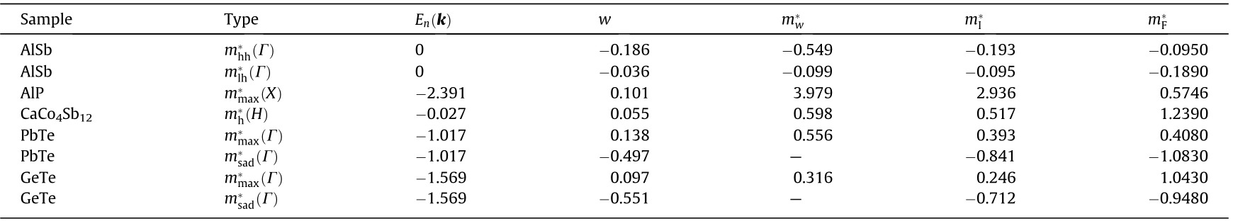
It is found that, overall, there are a considerable number of critical points, and warped critical points are not uncommon. Fig. 4 shows a typical BZ for FCC GeS (included in Table S5 in Appendix A). The plotted shapes display 18 critical point locations. Each critical point also has several symmetry-related neighbors that are determined by the point group at the location of the given critical point. In this case, there are 307 critical points in total, including all symmetries (but discounting critical points at the same k but different energy). We found that 57% of the critical points identified in our search were saddle points that manifest as van Hove singularities in the DOS [3]. In the case of a saddle point, the eigenvalues of M* have a different sign. The DOS effective mass obtained using Eqs. (13) and (14) diverges for a hyperbolic IEMS and is not calculated. The calculations of the DOS effective mass determined via the fitting procedure and via second-order derivatives are numerically equivalent in cases where band warping does not occur. Where warping occurs (e.g., in Table 2), there is a large difference between the fitting procedure and the Fourier derivative method, since the warping effects prevent the energy from being Taylor expanded in three dimensions. We found that band warping only occurred at critical points with degenerate energy eigenvalues, and we did not find any band warping at isolated nondegenerate critical points. Fig. 5 shows an example of the band structure of silicon (Si), with the critical points marked with red points and the degree of warping noted as red disks. The magnitude of the warping parameter is indicated by the diameter of the disk. It can be seen that the valence band is warped, albeit mildly with respect to some of the other critical points, whereas the conduction band minimum along  is not warped. Table 2 shows a sample of some representative warped critical points. The warping parameter gives a measure of the degree of warping. With zero warping, the critical point is ellipsoidal or hyperbolic, and the DOS effective masses from the other two methods (
 I and
I and  ) agree with the warped calculation (). However, it can be seen that the values of the direct fit () and Fourier derivative () method do not agree with each other at warped critical points. This is to be expected, since the fit will depend on the choice of coordinates at a non-analytic point. The failure stems from the fact that the IEMS cannot be fit to an ellipsoidal surface at a warped point. The warping parameter, as defined in Ref. [5], is computed for all critical points and determines whether a fitting procedure to an ellipsoidal form is appropriate.
《Fig. 4》
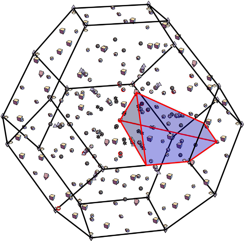
Fig. 4. Critical points for FCC GeS in the first BZ. Each polyhedral shape relates to a different symmetry (star of the k-point) of the BZ, depending on the location of a representative point.
《Table 2》
Table 2 Warping extent w and DOS effective mass at selected warped critical points calculated with 3 different methods: integral over the IEMS, ellipsoidal fit of the IEMS, and secondorder Fourier derivative. The table includes the following critical points: heavy-hole band (m*hh) and light-hole band (m*lh) at = (0, 0, 0) , the maximum of the valence band (m*max) at X = (1, 0, 0) or , and selected saddle point (m*sad) at .
Note: For saddle points, the warped DOS effective mass is unavailable. The fit and Fourier () methods for computing the components of the effective mass are only valid when the IEMS is not warped (ellipsoidal or hyperboloidal). When the IEMS is warped, then the fit and Fourier method fail and the m* calculated with those methods differs from the correct value of .
《Fig. 5》
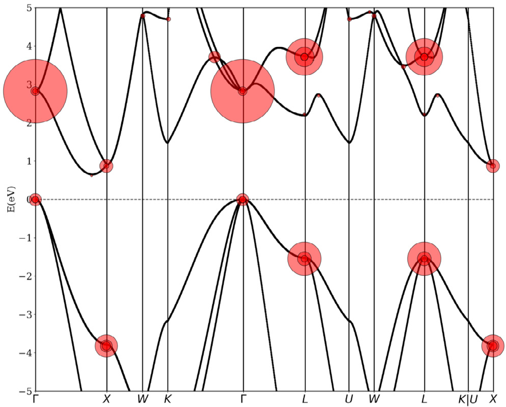
Fig. 5. An example of the Si band structure computed along the path suggested by Ref. [1] without spin–orbit coupling and with warping noted in red circles. The magnitude of the warping parameter w, is given as the size of the disk.
Consider Fig. 6 where the relative error of the direct fitting relative to the warped DOS effective mass is plotted versus the warping parameter. It can be seen from the figure that there is a general positive correlation, indicating that the warping parameter is a measure of how badly traditional methods (e.g., direct fitting or the Fourier method) perform when evaluating effective masses; thus, the warping parameter is an indication of how badly a Taylor approximation will perform in approximating the surface of an IEMS at a warped point. This is similar to what is reported in Ref. [6] for a surface warped in Kittel’s form. Thus, the only correct value for the DOS effective mass is . Fig. 7 shows the DOS of CaCo4Sb12. Critical points (van Hove singularities) are marked as red disks. The size of the disk indicates the amount of warping, as calculated in Ref. [5]. It can be seen that the DOS effective masses give rise to the shape of the non-smooth points. The particular shape can be expressed in terms of the DOS effective mass [4,6]. With spin–orbit coupling included, the largest warping value w is about 1.94 in CaCo4Sb12 at . In general, without spin–orbit coupling, there are many more warped points (since spin–orbit coupling lifts degeneracy), and the warping is larger in that case. This study provides a computational answer to questions related to the origin and occurrence of warping effects [60]. Without exception, warping did not occur at a specific critical point without the presence of degeneracies.
《Fig. 6》
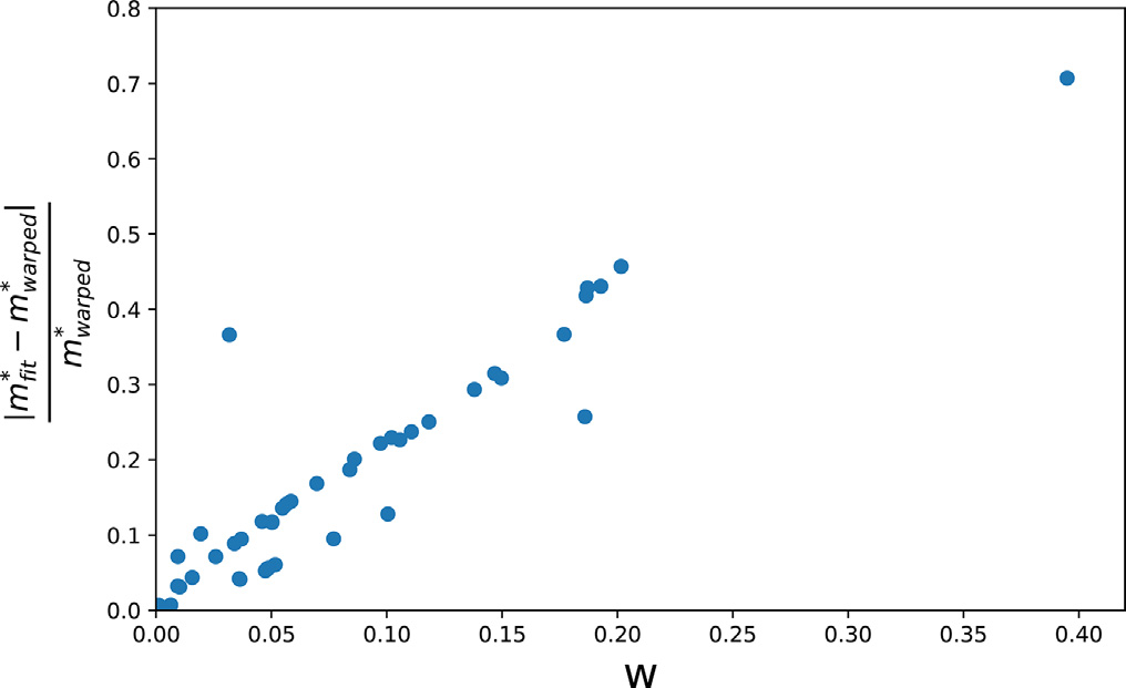
Fig. 6. The error between the warped effective mass DOS calculation and the DOS effective mass calculated with the fit to the IEMS versus the dimensionless warping parameter (w), for the materials in this study.
《Fig. 7》
Fig. 7. DOS for CaCo4Sb12 including spin–orbit coupling. The van Hove singularities are identified by red disks, where the diameter of the disk is determined by the warping parameter of the critical point located at the center of the disk. The shapes of the IEMS at the warped critical points are included in the figure. Blue (red) portions of the IEMS represent negative (positive) band curvature.
In all of the cubic materials, all saddle points at and at L (or other critical points) are warped. The reason for this can be seen in the requirements placed on the IEMS: The IEMS will have regions of positive and negative values due to the saddle behavior of the energy dispersion, and the cubic symmetry forces the principal directions to be the same. These two competing geometric requirements lead to warping at these points.
The HT list of critical points and effective masses has a variety of applications. For example, a full approximate analytic model of the BZ may be accomplished by approximating each critical point with the corresponding ellipsoid or saddle in the case of materials where warping is not an issue for critical points near the Fermi energy. This could be used for calculating scattering rates in Monte Carlo simulations [7] or for calculations of relaxation times [61] for different scattering processes. Moreover, a full analytic band structure would allow for possible band engineering, for the exploration of material properties, and even for the low-dimensionality reduction of thermoelectric properties [62]. A full description of the effective masses would also provide a model for the exploration of anisotropic transport considerations. As opposed to critical points that are not near high-symmetry points, lines, or planes, none of the effective masses from a quadratic expansion of the energy dispersion need to be the same. This gives rise to anisotropic transport that is all but ignored to avoid excessive complication. This procedure provides examples where anisotropy may be relevant for transport or other properties and provides a first step toward realistic analytic descriptions of band structures with these properties.
The Appendix A includes: ① the Hubbard U correction determined with the ACBN0 self-consistent protocol (Tables S1, S4, S14, and S18); ② characterization of the critical points found in the proximity of the Fermi level for AlSb, AlP, GeS, GeSe, GeTe, PbS, PbSe, PbTe, SnS, SnSe, SnTe, CoSb3, CaCo4Sb12, BaCo4Sb12, Bi2- Se2Te, Bi2Te3, Bi2Te2Se, Bi2Se3, Bi2Te2S, and Bi2Se2S (Tables S2, S3, S5, S7–S13, S15–S17, S19–S24); and ③ band structure plots (Figs. S1–S20).
《4. Conclusions》
4. Conclusions
We have designed and applied a two-level HT calculation with the aim of finding and characterizing critical points in the BZs of several materials. This search identified features of the band structures,  , that are not visible in 2D plots but nonetheless contribute to electronic transport, DOS, and other material properties. We used three different methods to compute the DOS effective masses at these critical points: namely, the direct method, the Fourier derivative method, and the warped method. At analytic (ellipsoidal) critical points, all approaches agreed with each other and aligned well with literature values, where available. This study also identified many warped critical points and used Eqs. (13) and (14) to correctly calculate the DOS effective mass. At these warped points, we provided reliable values for
  using the theory reported in Ref. [5]. All three methods disagreed, but the ‘‘warped” method was correct. Standard 2D band structure plots are often inadequate to convey the complicated nature of the effective masses at important critical points. Our HT procedure overcomes this issue and facilitates comparison with experiments and the development of analytical models, as well as band structure engineering and the tuning of properties for technological applications.
《Acknowledgments》
Acknowledgments
The authors would like to thank Lorenzo Resca for helpful discussions regarding the symmetry properties of the Brillouin zones, along with other aspects concerning warping. This work was performed in part through computational resources and services provided by the Institute for Cyber-Enabled Research at Michigan State University. Nicholas A. Mecholsky would like to acknowledge financial support from the Vitreous State Laboratory.
《Compliance with ethics guidelines》
Compliance with ethics guidelines
Andrew Supka, Nicholas A. Mecholsky, Marco Buongiorno Nardelli, Stefano Curtarolo, and Marco Fornari declare that they have no conflict of interest or financial conflicts to disclose.
《Appendix A. Supplementary data》
Appendix A. Supplementary data
Supplementary data to this article can be found online at https://doi.org/10.1016/j.eng.2021.03.031.


 京公网安备 11010502051620号


