

《1. Introduction》
1. Introduction
Over the past decade, data-driven intelligence has been rapidly pushing the envelope in the construction of complex industrial processes by taking advantage of the Industrial Internet of Things (IIoT), big data analytics (BDA), and artificial intelligence (AI) technologies [1–3]. In this context, in order to better create products and services from various materials and resources, the performance of complex industrial processes should be further improved in areas such as product quality, production efficiency, energy consumption, and pollutant emissions. However, these key performance indicators (KPIs) usually cannot be measured and analyzed online through existing sensors [4,5]. Offline laboratory analysis introduces high delay, making it challenging to improve industrial production in time [6,7]. Therefore, the soft sensor technique has attracted extensive efforts for the online estimation of industrial KPIs.
The soft sensor technique aims to describe the input–output behavior of the system by constructing mathematical models with easy-to-measure variables as the input and KPIs as the output. It can be roughly classified into two categories: first-principle (white-box) models and data-driven (black-box) models [8,9]. Models in the former category represent the causality of actual systems, which can only work well by a prior understanding of the physical or chemistry knowledge [10,11]. As a result, data-driven models, which focus on association relationships without reflecting actual causality, have become the mainstream to develop soft sensors for industrial KPIs [12].
For example, shallow machine learning (ML) models, such as partial least-squares (PLS), support vector regression (SVR), and their extensions, have been employed to learn quality characteristics from the historical data of complex industrial processes. In Ref. [13], an optimized sparse PLS (OSPLS) model is proposed to estimate the product quality of batch process industries. A robust multi-output least-squares SVR (M-LS-SVR) has been proposed for the online estimation and control of molten iron quality indices in blast furnace ironmaking [14]. Furthermore, deep learning (DL) models have been widely studied to capture nonlinear features in complex industrial data. Aiming for multisource heterogeneous data, Ren et al. [15] proposed a wide–deep–sequence (WDS) model combining a wide–deep (WD) model and a long short-term memory (LSTM) network to extract quality-related information from both key time-invariant variables and time-domain features. Yuan et al. [16] developed a sampling interval-attention LSTM (SIALSTM) to deal with time series with irregularly sampled data in the soft sensing of key quality variables. Ou et al. [17] proposed a stacked autoencoder (SAE) with quality-driven regularization for quality prediction in an industrial hydrocracking process. To reduce the information loss and generalization degradation of DL models, Yuan et al. [18] proposed a layer-wise data augmentation-based SAE (LWDA-SAE) for the soft sensing of boiling points in the hydrocracking process. Considering the issue of input feature selection in DL, Wang et al. [19] proposed a multiobjective evolutionary nonlinear ensemble learning model with evolutionary feature selection (MOENE-EFS) for silicon prediction in blast furnace ironmaking. Furthermore, in Ref. [20], a deep probabilistic transfer learning (DPTL) framework is proposed to tackle the distribution discrepancy and missing data in a multiphase flow process. Although the above methods have achieved acceptable results in some industrial applications, there are still some research gaps.
Feature selection is still a crucial issue, because a raw industrial dataset is usually high-dimensional, and not all features are conducive to the development of soft sensors. Data-driven soft sensor modeling is essential to recognize patterns in industrial data, so as to determine the quantitative relationships between industrial KPIs and their related features (variables). Selecting a compact and informative subset of features can greatly reduce the complexity of models and help us to fully understand the operation mechanisms of complex industrial processes [21–23]. If the selected features are the causal variables of KPIs, data-driven soft sensors will undoubtedly be more interpretable and stable. Otherwise, blindly improving data-driven models will introduce a complex model structure and difficult-to-tune hyperparameters, which are contrary to the principle of Occam’s Razor and the reliability requirements of industry [24]. In other words, it is preferable for a feature-selection method to automatically select a subset of features for soft sensor modeling in which each feature has a unique causal effect on industrial KPIs.
Furthermore, actual industrial data is difficult to obtain and expensive, especially for discrete industries, which hinders the industrial applications of data-driven soft sensors. Based on the production behaviors, complex industrial processes can be classified into process and discrete industries [25]. The production behaviors of the process industries are either continuous, such as chemical processes, power generation, and ironmaking, or occur on a batch of indistinguishable materials, such as food processing, paper making, and injection molding. The production behaviors of discrete industries are either physical or mechanical processes for materials, such as engine assembly, semiconductor manufacturing [26], and household appliance manufacturing, in which the materials used are usually the products of other industrial processes [27,28]. Such processes usually have a larger scale, stronger dynamic, and less clear mechanism than those of process industries. The data collection depends almost entirely on the experience of industrial practitioners, so the raw industrial data is more nonlinear, insufficient, and uncertain. In this situation, ensemble ML with fewer parameters, good robustness, and interpretability is more suitable for complex industrial processes with weak mechanisms [29].
Therefore, this study focuses on the following two scientific questions: ① How can the causal effect between each feature and the KPIs in a raw industrial dataset be quantified? ② How can a subset of features for data-driven soft sensor modeling be automatically selected? Causal models such as the Granger causality, the conditional independence test, and structural equations [30–32] have been widely employed for research on finance [33], climate [34], and industry [35–37]. However, there is no research on integrating causal effect and feature selection for data-driven soft sensors. The main challenges are as follows. The conditional independence test will lead to information loss for the soft sensing of KPIs because of the data adequacy assumption. In addition, the Granger causality and structure equation models depend on the hypothesis of the data-generation mechanism. In summary, the main works of this study are listed below.
(1) Inspired by the post-nonlinear causal model, we integrate it with information theory to quantify the causal effect between each feature and the KPIs in a raw industrial dataset. This can avoid the hypothesis of the data-generation mechanism and provide helpful insight for understanding complex industrial processes.
(2) A novel feature-selection method is proposed to automatically select the feature with a non-zero causal effect to construct the subset of features, which can reduce information loss, promote the interpretability of soft sensor models, and help to improve accuracy and robustness.
(3) The constructed subset is used to develop soft sensors for the KPIs by means of an AdaBoost ensemble strategy. We also introduce two actual complex industrial processes: an injection molding process from Foxconn Technology Group in China and a diesel engine assembly process from Guangxi Yuchai Machinery Group Co., Ltd. in China. Experiments on these two industrial applications confirm the effectiveness of the proposed method.
The rest of this paper is structured as follows. Section 2 describes related works. Sections 3 and 4 then provide detailed descriptions of the proposed method. Subsequently, in Section 5, experimental studies are carried out on two actual complex industrial processes. Finally, Section 6 summarizes the conclusions.
《2. Related works》
2. Related works
This section reviews feature-selection and causal discovery methods, which will motivate the problem formulation and basic idea of this study.
《2.1. Feature-selection method》
2.1. Feature-selection method
As circulated in the industry, data and features determine the upper limit of ML, while models and algorithms just approach this upper limit. Feature selection involves selecting a subset of features as the input of ML from a given candidate feature set [38] and is motivated by two reasons. First, even if there is no a priori or domain knowledge, feature selection helps us to fully understand the data and provides perceptual insights [39]. Second, it directly realizes feature dimensionality reduction, which effectively reduces the complexity of ML models [40]. In general, two key aspects are involved in feature selection: the subset search strategy and subset evaluation criteria.
2.1.1. Subset search strategy
Take a candidate input feature set F with M input features, where F = {X1, X2, ..., XM}, and Xi (i is the number of X and i = 1, 2, ..., M) denotes the candidate input feature. There are 2M candidate subsets S, where S  F. The objective of the subset search strategy is to select an optimal feature subset S from F [41]. Eq. (1) shows that the forward search strategy first initializes S with an empty set. After that, based on the subset evaluation criterion, one feature is selected from F and added to S in each iteration until the stopping threshold is reached.

where EC(·) denotes the evaluation criterion; ST denotes the stopping threshold; and Y denotes the output feature.
Another strategy is called backward search, as illustrated in Eq. (2); this first initializes S = F. Then, one feature is removed from S in each iteration until the stopping threshold is reached.

These two strategies are greedy because only the local optimality is implemented. Moreover, it is difficult to determine the optimal evaluation criteria and stopping threshold with good interpretability and theoretical basis.
2.1.2. Subset evaluation criteria
Many evaluation criteria have been used to judge whether to retain the candidate feature in each iteration, such as the degree of association and divergence, and the performance of ML models. The variance σ2 measures the degree of feature divergence, and does not consider the association between input and output features [42]. The Pearson correlation coefficient (PCC) selects the input features most relevant to the target, and only focuses on the linear association [43]. The maximal information coefficient (MIC) detects the nonlinear association between two variables [44], but more samples are needed, and the total association is easy to underestimate. Feature selection based on the above criteria does not depend on ML models and is also known as a kind of filtering method.
The parameters of ML models, such as the information gain of a decision tree and regression coefficients [45], can also be used as subset evaluation criteria, which measure the importance or weight of features. This kind of method, which is known as embedding, relies on an ML training process with expensive computing costs and is essentially based on associations. Aside from taking the performance maximization as the evaluation criteria, wrapper methods combine ML with optimization algorithms, such as genetic [38], evolutionary [19], and particle swarm algorithms [39], to automatically select optimal feature combinations. Wrapper methods also bring expensive computing costs, and it is easy to cause over-fitting, especially in industrial applications.
《2.2. Causal discovery method》
2.2. Causal discovery method
Discovering causal relations is a fundamental task of scientific research and technological progress; it strictly distinguishes cause and effect variables, revealing the mechanism and guiding decision-making more effectively than an understand of associations can do. Without considering the lagged effect, causal discovery approaches mainly rely on conditional independence tests and structural equation models to learn causal effects from observed data [46].
2.2.1. Conditional independence tests
Given a set of ternary variables {X, Y, Z}, the specific causal structure can be tested by the conditional independence between variables. As illustrated in Fig. 1, if the relation between ternary variables is that Y, X, and Z are independent, then the causal structure must be Markov equivalent class (Fig. 1(a)). If the relation is that X and Z are independent on their own, but are not independent once Y is introduced, the causal structure must be a Vstructure (Fig. 1(b)). On this basis, Peter–Clark (PC) and inductive causation (IC) algorithms, which are suitable for a wide range, learn causal structure through a two-stage process of the causal skeleton and causal direction [47,48].
《Fig. 1》
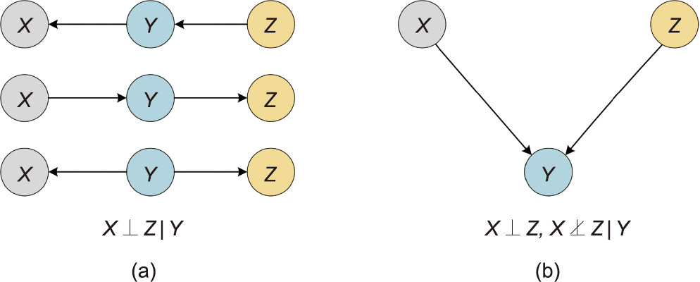
Fig. 1. Causality between ternary variables. (a) Markov equivalent class; (b) Vstructure.
2.2.2. Structural equation models
The hypothesis of the data-generating mechanism describes how the effect variables are determined by causal variables and causal mechanisms, including the linear non-Gaussian acyclic model (LiNGAM) [49], the additive noise model (ANM) [50], information geometric causal inference (IGCI) [32], and the postnonlinear model (PNM) [51]. As the most general model, illustrated in Fig. 2, PNM includes the nonlinear influence  of the cause X, the noise or disturbance ε, and the measurement distortion
  in the observed effect Y. The formula is shown below.

where  X; and are nonlinear functions, and should be invertible.
Due to the limitations of data sufficiency and conditional independence tests, the causal structure obtained from the PC and IC algorithms is not equivalent to the actual physical object. Feature selection based on this causal structure will cause significant information loss, so that the best feature combinations for ML are not attained. In contrast, the PNM in structural equation models can more effectively bridge causal discovery and feature selection.
As for the feature-selection issue, embedding and wrapper methods rely on an ML training process with expensive computing costs. Their performance is directly affected by the selected ML models. Filtering methods, such as variance-based, PCC-based, and MIC-based methods, do not depend on ML models and select a subset of features by manually setting a stopping threshold in advance. A typical stopping threshold includes a specific number of selected features, such as a specific variance value, PCC value, or MIC value. Obviously, it is difficult to determine a stopping threshold with good interpretability and a theoretical basis. Causal discovery brings new light to solve this problem by quantifying the causal effect between each feature and the KPIs in a raw industrial dataset to automatically select a subset of features for data-driven soft sensor modeling. The proposed method is introduced in detail in the next section.
《Fig. 2》
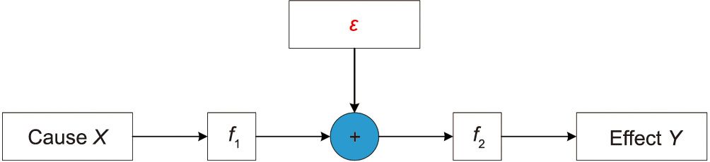
Fig. 2. Post-nonlinear causal model. , : nonlinear functions; ε: the noise or disturbance.
《3. Causal model-inspired feature selection》
3. Causal model-inspired feature selection
《3.1. PNM with information theory》
3.1. PNM with information theory
Given a set of cause variables {X1, X2, ..., Xk} (where k is the number of variables) and effect variable Y, the PNM in Eq. (3) can be extended to Eq. (4).

To discover the causal relations between another variable Xk+1 and Y, Eq. (4) is further extended to Eq. (5).

If Xk+1 reduces the noise term, it contains the causal information of Y. Thus, the causal effect of Xk+1 on Y can be quantified by Eq. (6).

where CE is causal effect.
The problem is that it is necessary to establish and depend on the two regression models, which have high computational complexity and affect accuracy. In addition, the hypothesis of the data-generating mechanism in PNM should be improved.
This study defines the causal effect by means of information theory to solve these problems. In information theory, the Shannon entropy is adopted to measure uncertainty and average information in a discrete random variable X as follows:

where H(·) denotes the Shannon entropy; P(x) denotes the probability mass function; and x is the observed value of X.
The total uncertainty in the two discrete random variables X and Y can be calculated by joint entropy as follows:

where y is the observed value of Y.
If X is given, the uncertainty in Y can be reduced by considering the information in X. Then, the residual uncertainty in Y can be calculated by conditional entropy as follows:

By substituting Eqs. (7) and (8) into Eq. (9), the conditional entropy can be presented by the probability of X and Y. Information theory extends PNM by considering uncertainty instead of variance [30]. In other words, the causal effect can be quantified by measuring the extent to which Xk+1 reduces the uncertainty of Y. As illustrated in Fig. 3, given a set of cause variables {X1, X2, ..., Xk}, the residual uncertainty in Y can be calculated by

When Xk+1 is further given, the residual uncertainty in Y can be represented as follows:

Thus, the causal effect of Xk+1 on Y is obtained as follows:

Eq. (12) only relies on the information theory to realize regression model-free causal effect quantification. Furthermore, data discretization is a vital data preprocessing technique to calculate the entropy of continuous random variables. In this study, we apply a histogram-based method to discrete data, and the optimal number of bins nh is estimated by

where R is the range of data; IQR is the interquartile range; and n is the number of samples.
《Fig. 3》
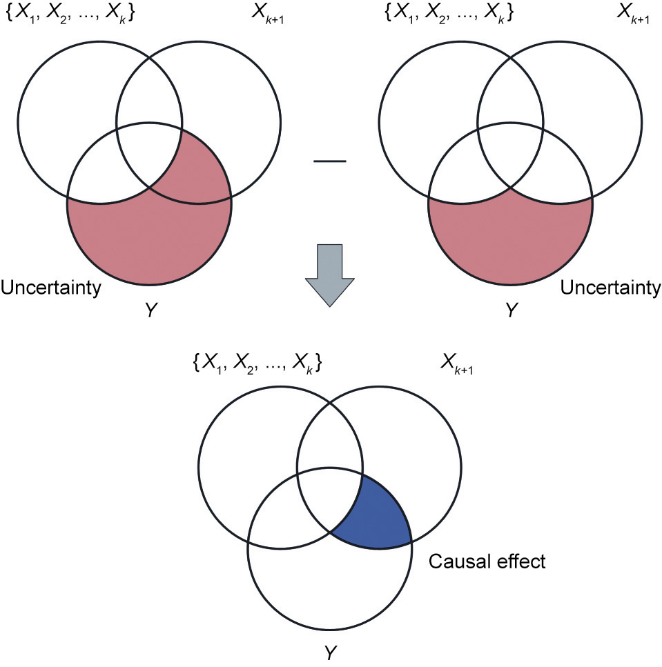
Fig. 3. Venn diagram of the improved causal effect, where the first red shadow indicates the residual uncertainty in Y when a set of cause variables {X1, X2, ..., Xk} is given, the second red shadow indicates the residual uncertainty in Y when Xk+1 is further given, and the blue shadow indicates the causal effect of Xk+1 on Y.
《3.2. Causal effect-based automatic feature selection》
3.2. Causal effect-based automatic feature selection
We present a novel feature-selection idea that takes the forward search strategy as the subset search strategy and the causal effect in Eq. (12) as the subset evaluation criteria. Its formal expression is as follows:

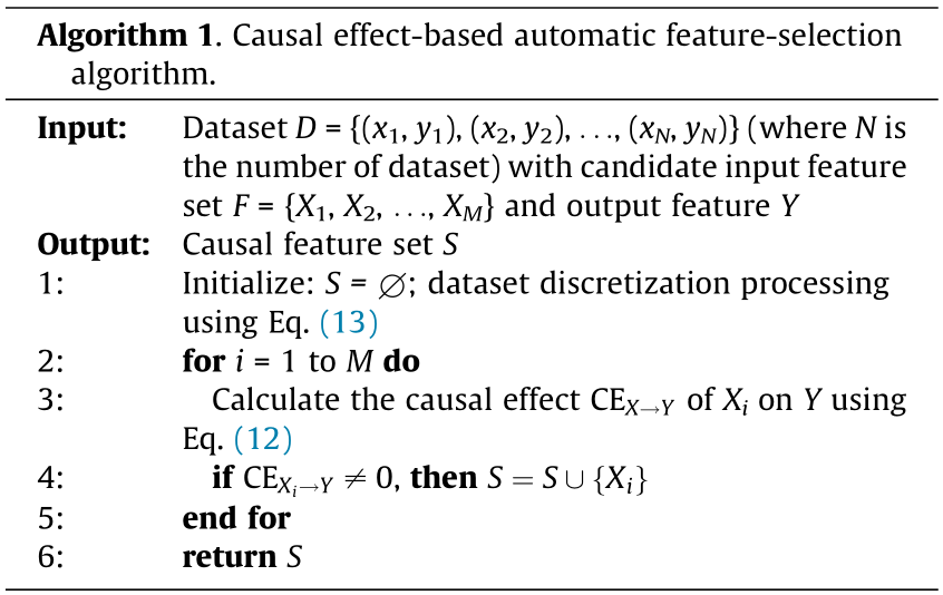
Compared with Eqs. (1) and (2), the feature-selection method shown in Eq. (14) only needs to traverse all candidate input features Xi in a specific order, does not need to set a stop threshold, and automatically selects the input feature combination with a non-zero causal effect. In the actual execution process, we determine the traversal order according to the mutual information between each candidate input feature Xi and output feature Y. Algorithm 1 gives the pseudo-code of the causal effect-based automatic feature-selection algorithm. The detailed implementation process of this method is also shown in Fig. 4.
《Fig. 4》

Fig. 4. Flow chart of the proposed method.
《4. AdaBoost decision tree-based soft sensor modeling》
4. AdaBoost decision tree-based soft sensor modeling
In this study, taking the decision tree as the basic learner, an AdaBoost ensemble ML algorithm is employed for the soft sensor modeling of industrial KPIs. It should be pointed out that this model is not designed to outperform all existing models. Instead, we believe that, once the causal information is extracted, datadriven soft sensors can achieve satisfactory accuracy and interpretability. In the future, we will study more advanced ML or DL models for data-driven soft sensors.
《4.1. Decision tree regressor》
4.1. Decision tree regressor
A decision tree regressor is mainly a classification and regression tree (CART) algorithm, which can solve classification or regression problems. Take training dataset D = {(x1, y1), (x2, y2), ..., (xN, yN)} (where N is the number of samples). When applying a CART to solve the regression problems, based on the idea of bisection recursive segmentation, the optimal segmentation variable j and segmentation point s are selected by using the square error minimization criterion, that is, the following equation is solved:
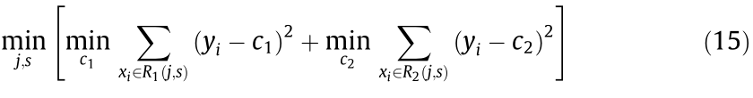
where c1 and c2 are output values; R1 and R2 are two regions in the input space.
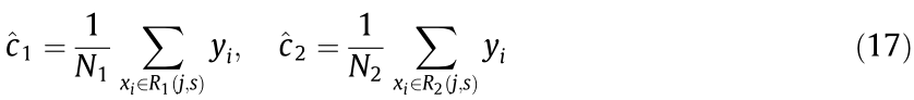
Then, the input space is divided into two regions R1 and R2 by the variable j and point s. Two sub-nodes are generated from this node, containing N1 and N2 samples, respectively.

The optimal output values  and
and  in these two regions are further determined as follows:
Let the process to recur in turn until the end conditions are met; finally, divide the input space into W regions R1, R2, ..., RW to generate a decision tree:
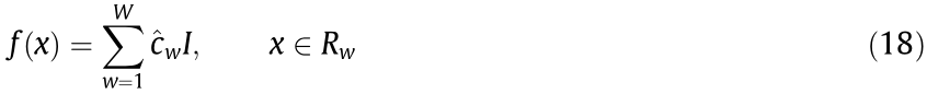
where I(·) is the indicating function and w is the number of regions. If x  RW, then I = 1; otherwise, I = 0.
After the regression tree is generated, it is pruned from the bottom to the root node. For each pruning case, a subtree is generated, thus forming a subtree sequence  . Next, use the cross-validation method on the independent verification data set to compare the square error of each subtree with respect to the verification set, and select the optimal decision tree
  (α is the number of sequence and α = 1, 2, ..., n).
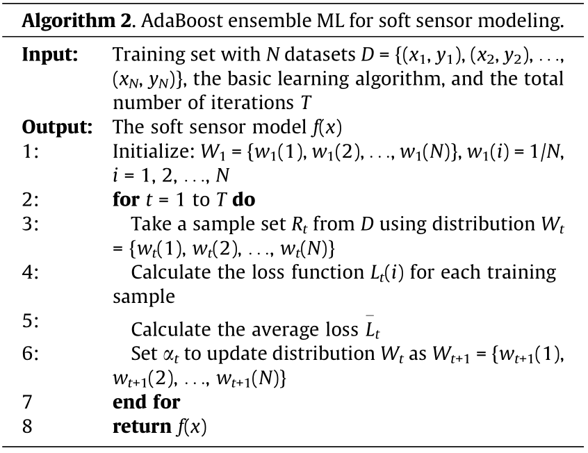
《4.2. AdaBoost ensemble learning for soft sensing》
4.2. AdaBoost ensemble learning for soft sensing
As illustrated in Algorithm 2, given D = {(x1, y1), (x2, y2), ..., (xN, yN)} as the training set, Wt = {wt(1), wt(2), ..., wt(N)} (t is the number of iteration and t = 1, 2, ..., T, where T is the total number of iterations) denotes the weight distribution over D at the tth boosting iteration. At later iterations, the weight distribution will be updated by increasing the weight of samples with poor performance and decreasing the weight of those with good performance. The average loss function to measure the performance is given by
where Lt is a loss function with a range of 0–1. Three candidate Lt are presented by Ref. [52]; this study uses the exponential one, as follows:

where  is the loss for each training example. The reweighting procedure is formulated as follows:

where  is the weight updating parameter; Zt is the normalization factor that makes Wt+1 a probability distribution. The final AdaBoost regression result can be obtained by
《5. Experimental studies》
5. Experimental studies
In this section, the proposed method is validated by experiments on two actual complex industrial processes.
《5.1. Experimental setup》
5.1. Experimental setup
According to the theoretical derivation, it can be seen that the proposed feature-selection method is a kind of filtering method. In this method, the causal effect is used as the subset evaluation criteria, and the forward search strategy is used to automatically select the subset of features for training the soft sensor model. The proposed method does not need to set a stop threshold. Each feature Xi in this subset has a unique causal effect on Y. It can be concluded without verification that other filtering methods lack this advantage.
The performance evaluation of feature selection usually considers two aspects: the number of selected features and the performance of the soft sensors. We hope to use the least number of input features to achieve the best performance of the soft sensors. It is well-known that variance-, PCC-, and MIC-based methods are the simplest and most effective filtering feature-selection methods with good generalization. Therefore, these three methods are taken as benchmarks for comparison purposes. We first use the proposed method to determine the number of selected features (marked as K). Then, the stop threshold of three benchmarks is also set to K. Finally, the feature subsets obtained by the above four methods are used to train the AdaBoost decision tree-based soft sensor model, and the performance of the soft sensors is compared. During this process, the experimental data of two complex industrial processes are randomly divided into two groups according to a 60:40 proportion; that is, 60% is taken as the training set and 40% is taken as the testing set. The root-mean-square error (RMSE) and the coefficient of determination R2 , which are two widely used performance evaluation metrics, are defined by Eqs. (23) and (24), respectively, and are adopted in this study. Eventually, if the RMSE and R2 of our method are better than those of the three benchmarks, the effectiveness of the proposed method can be verified.

where NT is the number of samples in the testing set; yi is the real value of the ith sample;  is the estimated value of the soft sensor model; and
  is the mean of all estimated values.
All the codes of this study are written in Python 3.7. The four most important hyperparameters of the AdaBoost decision treebased soft sensor model are the maximum depth and minimum samples split of each decision tree regressor, as well as the number of estimators and learning rate of AdaBoost ensemble learning. In two experiments, by fine-tuning up and down near the default value, they are set to 10.0, 5.0, 20.0, and 1.3, respectively. All other hyperparameters use default values. The hardware environment is Intel (R) Core (TM) i7-8700 central processing unit (CPU) @3.20 GHz 32.00G random access memory (RAM).
《5.2. Experimental study on the injection molding process》
5.2. Experimental study on the injection molding process
The first complex industrial process is the injection molding process from Foxconn Technology Group in China. This process uses an injection molding machine (Fig. 5) to melt the plastic raw materials at a high temperature. It then injects the plastic melt into the mold at high speed and high pressure; the melt undergoes complex physicochemical changes at a constant pressure to yield plastic products. Through the repeated operation of this process, a large number of the same products can be produced. During this process, the final product quality is measured with a high delay, which seriously affects timely decision-making for ensuring quality stability. Therefore, the injection molding process is used to verify and apply the proposed method. The data of 16 600 production batches were collected, including 86 candidate input features, and the product sizes were used as the KPIs [53].
《Fig. 5》

Fig. 5. Diagram of the injection molding machine.
Based on Section 3, we quantify the causal effects of 86 candidate input features on the product size (mm) of the injection molding process. As shown in Fig. 6, it is found that only nine candidate input features contain causal information about product size; given these nine features, the remaining features have no causal effect on it. Thus, these nine features are utilized as the input features of the soft sensor model to estimate the value of the product size. The nine features are: instantaneous flow (m3 ·s–1 ), cycle time (s), jacking time (s), post-cooling time (s), mold temperature (°C), clamping time (s), ejection time (s), clamping pressure (Pa), and opening time (s).
《Fig. 6》
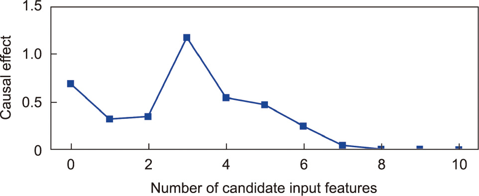
Fig. 6. The causal effect of different candidate input features on product size in the injection molding process.
Table 1 shows the RMSE and R2 of the soft sensor model under different feature-selection methods. We can see that the causal effect-based feature-selection method provides the lowest RMSE and the largest R2 . It outperforms the three benchmarks, because the causal information of product size is accurately extracted; in addition, redundant non-causal information is effectively removed. Moreover, compared with the benchmarks, the proposed method does not need to set a stopping threshold and can naturally avoid information loss.
《Table 1》
Table 1 RMSE and R2 of the soft sensing model under different feature-selection methods in the injection molding process.

Fig. 7 shows the soft sensor results for product size under different feature-selection methods. It can be seen that the causal effectbased method can more effectively estimate the slight fluctuation of quality than the methods based on three benchmarks. Fig. 8 shows the scatter diagrams and probability density curves of the soft sensor results under different feature-selection methods. It can be seen that the estimated values of the causal effect-based method are closer to the real value. Furthermore, the probability density curve from the causal effect-based method is ‘‘thinner” and ‘‘taller” than those from the benchmarks, which also proves that the proposed method has better accuracy.
《Fig. 7》

Fig. 7. Soft sensor results of product size under different feature-selection methods in the injection molding process. (a) Variance; (b) PCC; (c) MIC; (d) causal effect.
《Fig. 8》
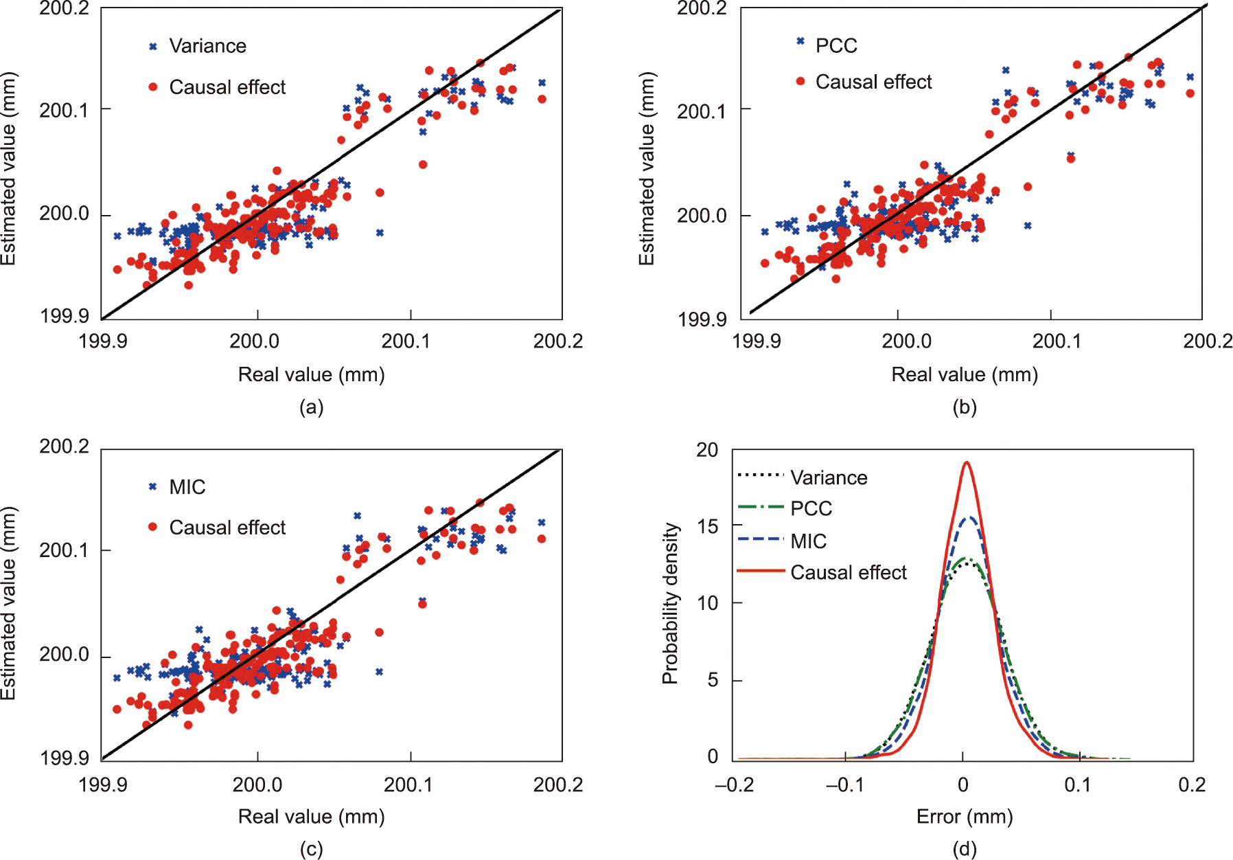
Fig. 8. Scatter diagrams and probability density curves of the soft sensor results under different feature-selection methods in the injection molding process.
《5.3. Experimental study on the diesel engine assembly process》
5.3. Experimental study on the diesel engine assembly process
The second complex industrial process is the diesel engine assembly process from Guangxi Yuchai Machinery Group Co., Ltd. (China). As shown in Fig. 9, mechanical parts are assembled into diesel engine products through eight sub-assembly lines, including the main assembly line, five sub-assembly lines, the performance test line, and the package line. The consistency of the rated power under the same work conditions is one of the most important KPIs, but its inspection requires time-consuming and high-cost bench testing. We implemented the test on 1763 samples; for each sample, the data of 39 process variables were collected along the assembly process [36,37] and were utilized as the candidate input features to verify and apply the proposed method.
《Fig. 9》
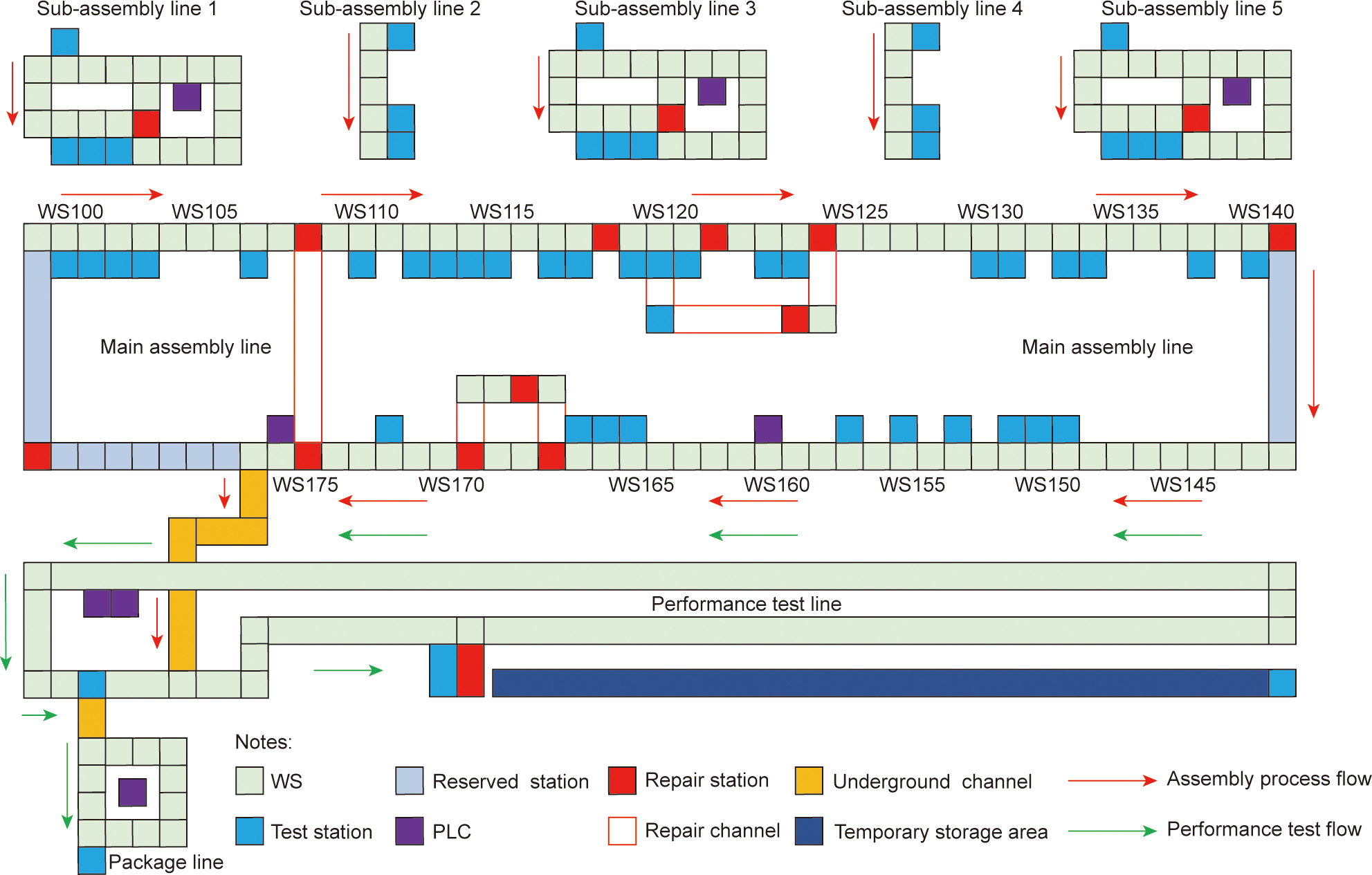
Fig. 9. Diagram of the diesel engine assembly process. WS: work station; PLC: programmable logic controller.
Further verification and application of the proposed method is performed on the diesel engine assembly process. Similarly, the causal effects of 39 candidate input features on the rated power (kW) of the diesel engine products are quantified. As shown in Fig. 10, it is found that only six candidate input features contain causal information about the rated power, while, given these six features, the remaining ones have no causal effect on it. Thus, these six features are utilized as the input features of the soft sensor model to estimate the value of the rated power. This six features are: fuel consumption per 100 kilometers (L), running time (min), fuel consumption rate (%), intercooler inlet pressure (Pa), intercooler inlet temperature (°C), and axial clearance (mm).
《Fig. 10》
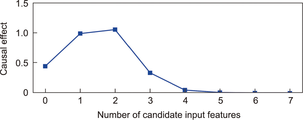
Fig. 10. The causal effect of different features on the rated power in the diesel engine assembly process.
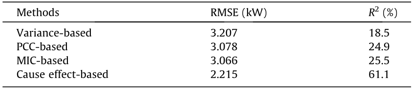
Table 2 shows the RMSE and R2 of the soft sensor model under different feature-selection methods. Again, we can see that the causal effect-based feature-selection method provides the lowest RMSE and the largest R2 . It is worth noting that the three benchmarks have very low R2 , indicating that it is difficult to explain the output features using the selected variables. Fig. 11 shows the soft sensor results for the rated power under different feature-selection methods. It can be seen that the causal effect-based method can more accurately estimate the value of the rated power than the three benchmarks. Fig. 12 shows the scatter diagrams and probability density curves of the soft sensor results under different feature-selection methods. The estimated values of the causal effect-based method are closer to the real rated power than those of the other methods. In addition, the probability density curve from the causal effect-based method is ‘‘thinner” and ‘‘taller,” which once again proves that the proposed model has better accuracy than the three benchmarks.
《Table 2》
Table 2 RMSE and R2 of the soft sensor model under different feature-selection methods in the diesel engine assembly process.
《Fig. 11》
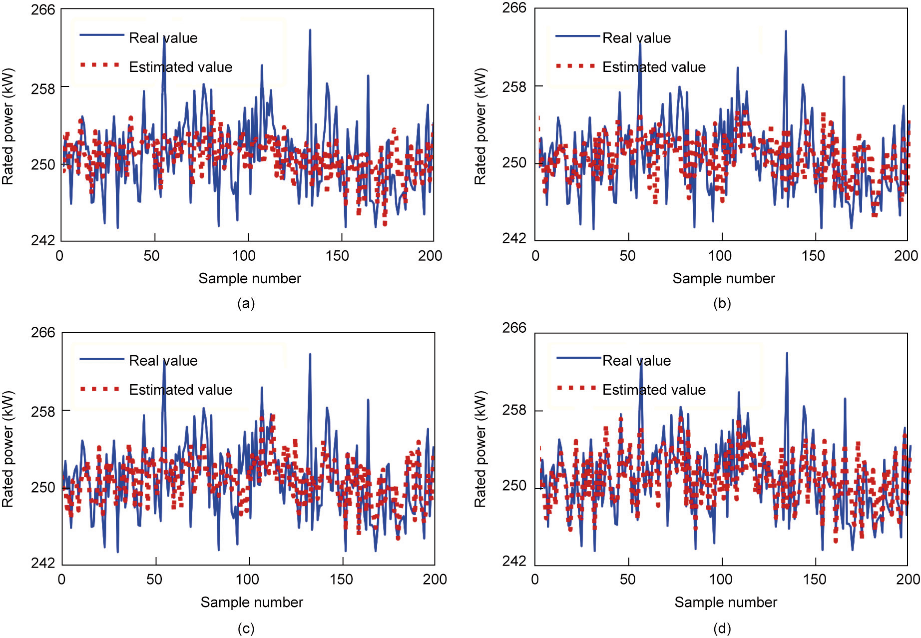
Fig. 11. Soft sensor results for product size under different feature-selection methods in the diesel engine assembly process. (a) Variance; (b) PCC; (c) MIC; (d) causal effect.
《Fig. 12》
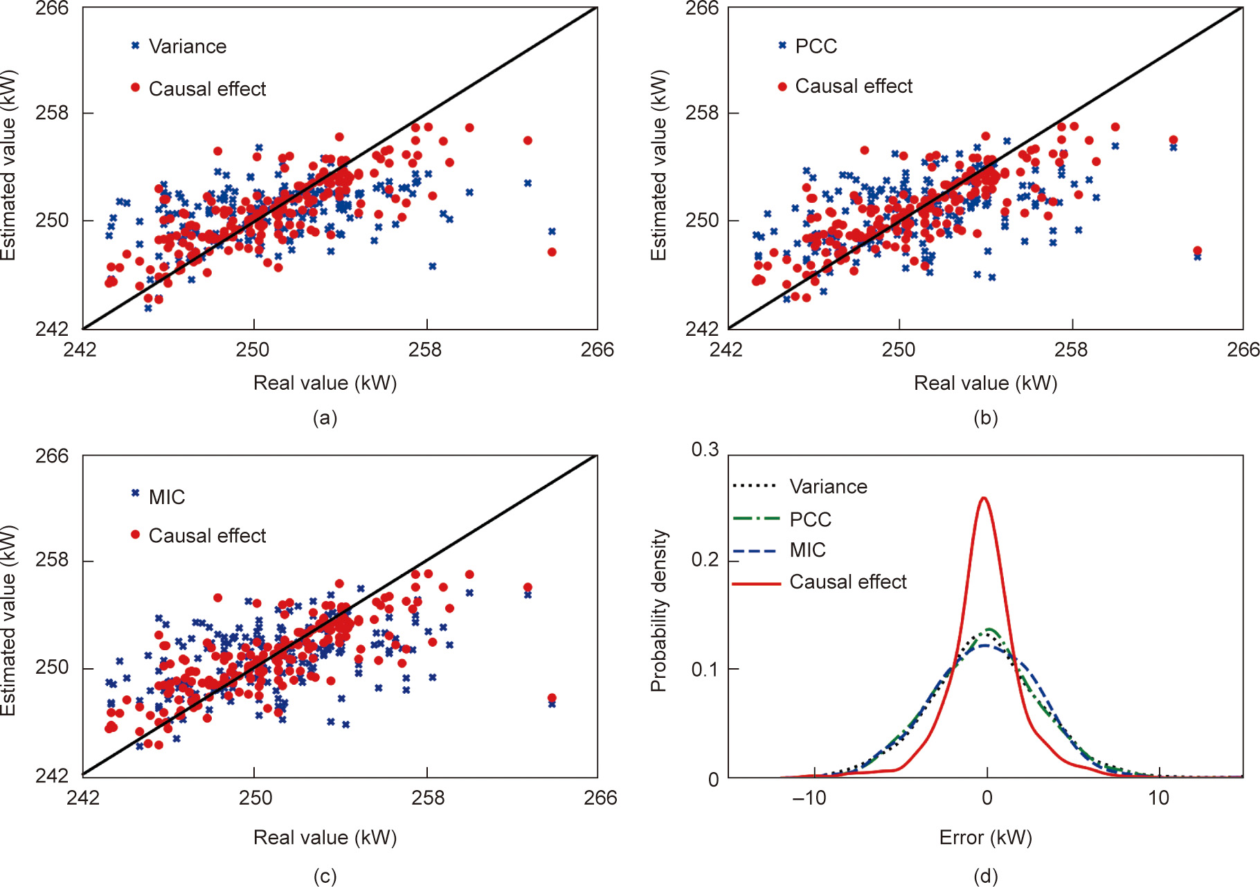
Fig. 12. Scatter diagrams and probability density curves of the soft sensor results under different feature-selection methods in the diesel engine assembly process.
According to the results of these two experiments, the following insights can be obtained. The proposed method is effective and universal, and can help us to understand complex industrial processes. In practical industrial applications, this method can select a subset of features from the raw industrial dataset that is compact and informative. For example, among the 86 candidate input features in the injection molding process, only nine candidate input features contain causal information about the product size. Compared with these nine features, other features are irrelevant or redundant for soft sensor modeling. The performance of the soft sensors can be further improved in two ways. One is to develop a more advanced data-driven model, which can fit the data distribution of the selected features more fully. Based on our experience, the performance of the existing data-driven models is similar when selecting the same input features. Thus, this paper only introduces an AdaBoost ensemble learning model for soft sensor modeling, while a comparison of different models lies beyond our scope. The other way is obtaining a deeper understanding of the industrial processes by means of first principles, so as to obtain more comprehensive and sufficient data to help train better datadriven models. In other words, although we are developing datadriven methods, research on the first principles of complex industrial processes should not be ignored.
《6. Conclusions》
6. Conclusions
This study proposes a causal effect-based feature-selection method for developing soft sensors for KPIs in complex industrial processes. Integrating the PNM with information theory, a causal effect quantification method is presented to extract the causal information of KPIs. The proposed method can provide helpful insights into the soft sensing of KPIs and helps to improve the accuracy and interpretability of ML. In addition, decision tree regression with the AdaBoost ensemble is employed for soft sensor modeling and requires almost no fine-tuning of parameters to achieve excellent performance. Our experimental studies on actual industrial processes confirm the effectiveness and promising applications of this method.
However, the PNM is a non-temporal causal model, so this paper does not consider the lagged effect of causality. If the proposed method is applied to time series data, it is necessary to first estimate the causal delay. This is another topic that may be addressed in our future work. In addition, this study focuses on the causal effect-based feature-selection method, while the research on downstream ML models is weak. As we mentioned earlier, under the same input features containing causal information, the improvement of soft sensor results by cutting-edge ML models is limited. Therefore, especially for complex industrial scenarios, our future work will focus on the interval estimation and risk assessment of KPI models based on the theory of uncertainty quantification.
《Acknowledgments》
Acknowledgments
We would like to thank the Ministry of Education–China Mobile Research Foundation Project of China (MCM20180703), and the National Key Research and Development Program of China (2020YFB1711100) for financial support. We would also like to thank Foxconn Technology Group for providing us with a historical dataset of the injection molding process, as well as the editors and reviewers for their valuable comments.
《Compliance with ethics guidelines》
Compliance with ethics guidelines
Yan-Ning Sun, Wei Qin, Jin-Hua Hu, Hong-Wei Xu, and Poly Z.H. Sun declare that they have no conflict of interest or financial conflicts to disclose.


 京公网安备 11010502051620号


