《1 Introduction》

1 Introduction

The concept of collective intelligence (CI) originated in 1785 with the Condorcet’s jury theorem, which states that if each member of a voting group has more than one half chance to make a correct decision, the accuracy of the majority decision in the group increases with the number of the group members [1]. In the late twentieth century, CI was applied to the machine learning field [2] and grew into a broader study of how to design collectives of intelligent agents to meet a system-wide goal [3,4]. This concept is related to the use of a single intelligent agent for reward shaping [5] and has been taken forward by many researchers in the game theory and engineering community [6]. However, while CI algorithms such as the well-known ant colony optimization (ACO) focused on how to make group intelligence emerge and go beyond the individual intelligence, they lacked a mechanism to evolve individual intelligence and could not be applied to a self-evolving artificial general intelligence (AGI) agent without significant extensions.

The long-standing goal of AGI has been to create programs that can learn for themselves from the first principles [7]. Recently, the AlphaZero algorithm achieved superhuman performance in the games of Go, Chess, and Shogi by using deep convolutional neural networks and reinforcement learning from games of self-play [8]. However, the reason for AlphaZero’s success has not fully been understood. Through analyzing and testing AlphaZero, we found that the logic of CI is implied in this algorithm. In this paper, we introduce the CI overview first. Next, we apply the AlphaZero algorithm to the game of Gomoku and observe the evolution power of the deep neural networks. After that, we compare Monte-Carlo tree search (MCTS) with ACO and identify MCTS as a CI algorithm. Finally, based on our analysis, we propose the CI evolution theory as a general framework toward AGI and apply the CI evolution theory to intelligent robots.

《2 Collective intelligence overview》

2 Collective intelligence overview

Recently, CI has been widely used in a variety of scenarios, such as the collaboration of the staff on a project, investment decisions of the board of a company and voting for presidential election. It seems that doing things by a group is more intelligent than that by an individual. However, Gustave Le Bon [8] pointed out in his famous book ‘The Crowd’ that group behavior can be extreme. In this sense, CI cannot be achieved by a simple combination of individuals. Therefore, we should first understand the features of CI to make the best use of it in achieving our goal.

In the field of sociology, a group of researchers (Thomas W. Malone et al.) from MIT Center for Collective Intelligence divided the required work into four components: executor, motivation, goal, and implementation parts. They then proposed ‘the CI genome’ based on this division [9]. Using Google and Wikipedia as examples, they analyzed these organizational genes systematically and presented the conditions for ‘CI genes’ to be useful. Moreover, their colleagues systematically studied the group performance in two different experiments and found the ‘C factor,’ which measures the group’s general ability [10]. This ‘C factor’ is correlated with the average social sensitivity of group members, the equality in discourse power, and the proportion of females in the group. Predictably, by recombining ‘CI genes’ and considering the ‘C factor’ in accordance with the task, one can get the powerful system he needs.

On the foundation of these sociological theories of CI, people have been able to better solve problems with the help of collective effort, especially in computer science. In 1991, M. Dorigo et al. [11] studied the food searching behavior of ants and proposed the ACO algorithm [12−14]. The basic idea of this algorithm is to choose the next node based on a pheromone until the proper solution is reached. In the ACO algorithm, the updating process of the information distribution of the pheromone is based on all searching tours in the current iteration, which can be understood as the emergence of the CI of ants. In this sense, the ACO algorithm has been successfully used in multiple problems, e.g., the traveling salesman problem (TSP) [15−16], data mining, and optimization of proportional–integral–derivative control parameters. In addition, scientists have proposed several useful CI algorithms, such as the particle swarm optimization algorithm [17], which simulates the food hunting of birds.

Apart from CI’s success in these optimization problems, learning from crowds can be a solution to challenges in the real-world application of machine learning when big data is involved. For example, labels for training in the supervised learning may be too expensive or even impossible for many applications to obtain [18]. Therefore, researchers have developed CI learning technology [19−22] to overcome this difficulty. In the next section, we will see the power of CI in dealing with large numbers of labels for board games. In our study, we attempt to solve industry problems with CI evolution theory in applications such as intelligent robots, and we have presented preliminary results for verification. We hope that our work can stimulate the study of CI in computer science and pave the way for connecting CI with deep learning and reinforcement learning.

《3 Discovery of CI in AlphaZero》

3 Discovery of CI in AlphaZero

In this section, we review the theory applied in AlphaZero [8], as well as previous versions AlphaGo Fan [23], AlphaGo Lee [24], AlphaGo Master [24], and AlphaGo Zero [24]. Then, the theory is conceptually analyzed from the point of view of CI. The theory is divided into two parts: 1) the representation of individuals by deep neural networks and 2) the evolution of individuals by reinforcement learning. Note that we discuss the details of MCTS in the next section to highlight the significance of it, because this is where CI emerges. Finally, we apply AlphaZero to a new game called Gomoku to demonstrate the applicability of AlphaZero.

《3.1 Review of the main concept of AlphaZero》

3.1 Review of the main concept of AlphaZero

In the view of real-time playing, AlphaZero employs MCTS to search for the optimal move. Because the time for a search is limited, it is difficult to consider all possible moves. As a result, the policy network is used to reduce the width of the search, and the value network is applied to reduce the depth of the search. The policy network serves as a prior probability, which provides higher probability for moves that may eventually lead to a win. The value network is treated as an evaluation function, which offers the prediction of game outcome without simulating the game to the end.

In the view of training, the policy and value networks are trained by a policy iteration algorithm from reinforcement learning. MCTS is regarded as the policy improvement operator, because the probability given by the search is better than that given by the policy network. Hence, the search probability is the training label for the policy network. The self-play based on MCTS is viewed as the policy evaluation operator, where the policy stands for the search probability because the move is based on the search probability. The game outcome is the training label for the value network. In the following section, CI will be utilized to analyze AlphaZero from a different view.

《3.2 Representation of individuals by deep neural networks》

3.2 Representation of individuals by deep neural networks

The capability of individuals limits their intelligence. If the individual capability is low, CI cannot be inherited by individuals, even if CI emerges. In AlphaZero, the individuals are represented by deep neural networks to increase the capability of individuals.

In AlphaGo, the policy network is used to provide the probabilities of the next move given the current state of the board, and the value network is used to offer the probabilities of winning the game given the current state of the board. In AlphaGo Fan, the neural networks are separated into the policy and value networks. There are 13 convolutional layers for each of the two networks. In AlphaGo Lee, the number of filters in each convolutional layer is raised from 192 to 256. From AlphaGo Master to AlphaZero, the policy and value networks are combined in a single network, and the number of convolutional layers is raised to 39 or 79, excluding policy and value heads. This comparison is summarized in Table 1. The performance of AlphaZero is distinctly better than the performance of AlphaGo Lee. In addition, it should be noted that the neural network in AlphaZero trained by supervised learning has comparable performance with AlphaGo Lee. This fact exhibits the contribution of the neural network in AlphaZero.

《Table 1》

Table 1. Comparison of structures of AlphaGo neural networks.

There are several reasons why the neural network in AlphaZero is superior. The first and most important one is the size of the network. We can find that the number of convolutional layers in AlphaZero is three times that in AlphaGo Lee, which means the number of adjustable weights in AlphaZero is also roughly three times that in AlphaGo Lee. This indicates that the capability of the network is significantly improved. Therefore, the network can be trained to learn the search probabilities generated by MCTS, which means the individuals can inherit the knowledge obtained by CI. Other reasons include: 1) the residual block decreases the training difficulty; and 2) the dual-network architecture regularizes the policy and value networks to a common representation and improves the computational efficiency.

《3.3 Evolution of individuals by reinforcement learning》

3.3 Evolution of individuals by reinforcement learning

Once individuals have the required capability, the next question is how to make them evolve. To make individuals continuously evolve, the direction of evolution has to be determined. In AlphaZero, the direction is found by the individuals’ own experience, namely reinforcement learning. As a result, the individuals keep evolving and finally surpass the performance of their previous versions and human experts.

In the earliest version AlphaGo Fan, the policy network is initially trained by expert knowledge. Then, the REINFORCE algorithm is employed to improve the performance of the policy network. In other words, the reinforced network is trained by the outcome of the game that is played by the policy network itself. In the next version AlphaGo Lee, the value network is trained from the outcomes of the games played by AlphaGo, rather than the games played by the policy network. This procedure is iterated several times. From AlphaGo Master to AlphaZero, not only is the value network trained from the outcomes of games played by AlphaGo, but the policy network is also trained from the search probabilities generated by AlphaGo. It should be noted that MCTS is employed to generate the search probability and make the move.

From the development of AlphaGo, we can conclude that reinforcement learning becomes the key of evolution, and the quality of self-generated labels determines the level of evolution. For the value network, when comparing AlphaGo Fan with the later versions, the main difference is the outcomes of the games, namely the labels for the value network. In the later versions, the labels become more accurate because they are generated by AlphaGo, which uses MCTS to make the move instead of the reinforced policy network only. For the policy network, from AlphaGo Master to AlphaZero, the search probabilities generated by MCTS are employed as the labels, rather than the policy network’s own moves guided by the game outcomes. This comparison is summarized in Table 2.

《Table 2. 》

Table 2. Comparison of the source of labels.

The reason why the labels generated by MCTS are better than those generated by the policy network is briefly explained next. MCTS involves multiple simulations to make one move. In each simulation, the policy network is used for prior probability, and the value is used for updating action-value. We can treat the policy and value network in each simulation as an individual, and the search probability becomes more precise as the number of individuals increases. Therefore, MCTS can provide the CI, namely, the search probability in this case. In [24], MCTS is viewed as a policy evaluation operator in reinforcement learning. However, the policy that was evaluated in that case is the search probability instead of the policy network, which is different from the original policy iteration algorithm. Therefore, it is more proper to consider MCTS as a CI algorithm than a policy evaluation operator. Additional information about MCTS will be presented further in this paper.

《3.4 Results of training in Gomoku》

3.4 Results of training in Gomoku

To demonstrate the applicability of AlphaZero, we used this technique in a new game called Gomoku, as well as in its variant Renju. The training results are presented further in this section. Note that some improvements were made to AlphaZero to adapt it to the rules of Gomoku and Renju. These improvements are beyond the scope of this paper and will be explained in a separate paper.

The training results of the improved AlphaZero in Gomoku are shown in Fig. 1. The first plot shows the performance of the improved AlphaZero. Note that we also implemented the AlphaGo Fan in Gomoku, and its performance is added for comparison. Elo ratings were computed from the evaluation games with various openings between different players using 1 second of thinking time per move. For AlphaZero, we used a single graphic processing unit for the neural network computation. The second plot shows the accuracy of the neural network at each iteration of self-play in predicting moves from the test-set. The accuracy measures the percentage of positions in which the neural network assigns the highest probability to the move. The third plot shows the mean-squared error (MSE) of the neural network at each iteration of self-play in predicting the outcome of the testset games. Similarly, the training results of the improved AlphaZero in Renju are shown in Fig. 2.

《Fig.1》

Fig. 1. Training results of the improved AlphaZero in Gomoku.

(a) Performance of the improved AlphaZero in Gomoku. The performance of the corresponding policy network is indicated by gray color. (b) Prediction accuracy on the test-set moves. (c) MSE on the test-set game outcomes.

《Fig.2》

Fig. 2. Training results of the improved AlphaZero in Renju.

(a) Performance of the improved AlphaZero in Renju. The performance of the corresponding policy network is indicated by gray color. (b) Prediction accuracy on the test-set moves. (c) MSE on the test-set game outcomes.

From these figures, we can see that the performance of AlphaZero is better than the performance of traditional engines based on expert knowledge. The policy and value networks gradually learn their own strategy from their own experience. This demonstrates that AlphaZero can be applied to more games with different rules. The generality of AlphaZero is inherited from the generality of the deep neural network representation method and reinforcement learning evolution approach. Moreover, the labels generated by MCTS provide the direction of evolution for the reinforcement learning. In the next section, CI will be used to explain the principles of MCTS.

《4 Analysis of ACO and MCTS》

4 Analysis of ACO and MCTS

ACO is one of the most representative CI algorithms, and MCTS is known as an efficient search algorithm for the decision processes. In this section, the basic approaches of ACO and MCTS are analyzed and applied to TSP. From the test results, some common features of ACO and MCTS are extracted and analyzed.

《4.1 TSP》

4.1 TSP

TSP is a combinatorial optimization (CO) problem and can be defined as follows [25].

Let V = {a, …, z} be a set of cities, A = {(r,s):r,s∈V} be the edge set, and δ(r,s) = δ(s,r) be the distance of the edge (r,s)∈A. The TSP is the problem of finding the minimal cost of a closed tour that visits each city once. The case where the cities r∈V are given by their coordinates (x_r, y_r) is also called the Euclidean TSP.

TSP is one of the well-known non-deterministic polynomial difficult problems, where the computational complexity is polynomial to the number of cities in the set V.

《4.2 ACO》

4.2 ACO

ACO [25−27] was first inspired by the foraging behavior of real ants to solve difficult CO problems, such as the TSP. When searching for food, ants initially explore the area surrounding their nest in a random manner. As soon as an ant finds a food source, it evaluates the quantity and quality of the food and carries some of it back to the nest. During the return trip, the ant deposits a chemical pheromone trail on the ground. The quantity of the deposited pheromone, which may depend on the quantity and quality of the food, guides other ants to the food source. Ants communicate with others via pheromone trails, which enable them to find the shortest path between their nest and food sources.

When solving the TSP, there are two major steps in each ACO iteration:

Simulation: Each ant generates a complete tour by making actions according to the probabilistic state transition rule, which governs the selection of the action proportionally to the transition probability,

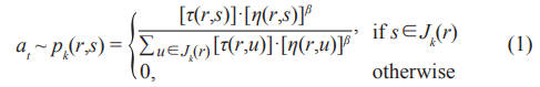
where τ is the pheromone, η = 1/δ(r,s) is the inverse of distance δ(r,s), Jk(r) is the set of cities that remain to be visited by ant k positioned at city r, and β is the parameter of the prior probability.

Update: Once all ants have completed their tours, a global pheromone updating rule is applied on all edges according to

where

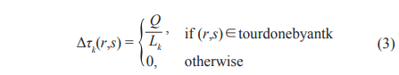
α is the pheromone decay parameter, L_k is the length of the tour performed by ant k, and m is the number of ants. Q is the weight parameter of pheromone, which determines the relative importance of exploitation versus exploration.

The process is iterated until the termination condition is met. In this paper, hyper-parameters Q = 1.0, α = 0.1, and β = 1.0 are used.

《4.3 MCTS》

4.3 MCTS

MCTS [28−30] is a heuristic tree search method for finding optimal actions in a given environment. MCTS has achieved great success in the challenging task of Computer Go. Combining MCTS with deep neural networks and self-play reinforcement learning, AlphaGo [23] and AlphaGo Zero [24] have succeeded in beating the best human players.

MCTS takes random actions as a simulation to estimate the value of each state in a search tree space. As more simulations are executed, the search tree grows larger, and the state values become more accurate. The tree policy used to select actions during the search is also improved by selecting children with higher values. Asymptotically, this policy converges to the optimal policy, and the evaluations converge to the optimal value function.

《Fig.3》

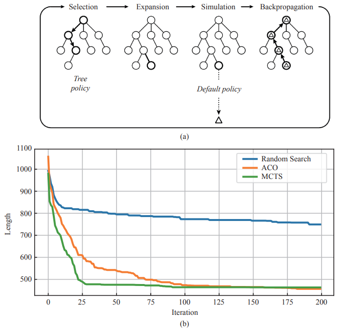
Fig. 3. (a) Four steps in each iteration of the general MCTS approach, and (b) convergence history of ACO, MCTS, and Random Search.

Fig. 3(a) shows one iteration of a general MCTS approach, and there are 4 steps [28] in every iteration:

Selection: Starting at the root node, a child selection tree policy is recursively applied to descend through the tree until the leaf node is reached. The tree policy in TSP selects the maximum action according to a variant of the upper confidence bound for trees (UCT) algorithm,

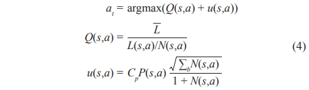
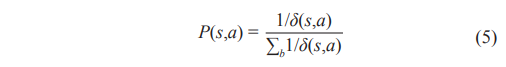
where s is the current node state, L(s,a) is the total route distance through edge (s,a), and N(s,a) is the number of times edge (s,a) has been visited so far. is the average length of all legal closed routes. Cp is the hyper-parameter, which determines exploitation and exploration of the tree. The prior probability is denoted by P(s,a), which is proportional to the inverse of the distance δ(s,a),

Expansion: To expand the leaf node, one (or more) child nodes are added to expand the tree according to the available actions.

Simulation: A simulation is run from the new node(s) according to the default policy to produce an outcome lt . The simulation default policy chooses a legal city proportional to the prior probability.

Backpropagation: The simulation result is backed up through the selected nodes to update their statistics,

After the specified number of iterations, the final action is chosen by selecting the most visited root child. In this paper, hyper-parameter Cp = 3.0 is used.

《4.3 Results and analysis》

4.3 Results and analysis

As the cities map in Euclidean TSP is an undirected graph, and the route is closed, the search graph can also be treated as a tree structure. In comparison with MCTS, ACO uses only one ant which starts from a fixed city in each iteration, and the fixed starting city is the root tree node in MCTS. The details of hyper-parameter settings are shown in Table 3.

《Table 3. 》

Table 3. Hyper-parameters in ACO and MCTS.

These two algorithms were applied to a 30-city TSP, and a random search with the MCTS default policy was added for the comparison. TSP optimization was run 10 times using these three methods, and the final results are shown in Table 4 and Fig. 3(b).

《Table 4.》

Table 4. Results of ACO, MCTS, and random search.

As we can see, ACO and MCTS both show a much better convergence than the random search. MCTS has a better convergence than ACO in the first 100 iterations; however, it stagnates in the latter half. One of the major reasons for this phenomenon is that the MCTS search structure is a tree, whereas the ACO search structure is a network. Thus, ACO still has better capacity in optimizing the local area.

Compared with ACO, MCTS has a similar mechanism of the optimization iteration. In an iteration, each individual needs to simulate according to the policy and update the global collective memory with the outcome. The simulation policy also evolves depending on the collective memory. Common features of these two methods can be listed as follows.

Simulation policy: In ACO, the simulation policy is given by the probabilistic state transition rule. In MCTS, the in-tree selection tree policy is the UCT algorithm, and the simulation policy is the default policy.

Collective memory sharing: In ACO, all simulation outcomes are updated with the pheromone, which determines the next simulation action probability. In MCTS, the simulation outcome updates with Q(r,s), which influences the next selection tree policy.

Balance between exploitation and exploration: In ACO, the simulation selects actions proportional to the state transition probability. In MCTS, the UCT algorithm is applied to balance the exploitation and exploration. To balance between exploitation and exploration, ACO has a hyper-parameter Q, while MCTS has a hyper-parameter C_p.

The listed features are also common features of CI emergence. From the test results and contrastive analysis, although MCTS does not have the explicit concept of population, the emergence mechanism can still be seen as a CI algorithm. The CI emergence is also the key reason for the efficient convergence of ACO and MCTS.

《5 Theory of the CI evolution》

5 Theory of the CI evolution

After a thorough study of the AlphaZero program and MCTS algorithm, the underlying intelligence evolution mechanism has been fully discovered. The success of AlphaZero relies mainly on two factors: 1) the use of a deep convolutional neural network to represent the individual intelligent agent, and 2) the use of MCTS to make group intelligence emerge and exceed individual intelligence. Deep convolutional neural networks are able to evolve their intelligence by training with proper target labels. The MCTS algorithm is able to generate proper target labels through the CI emergence. Combining these two factors in the reinforcement learning environment, a positive feedback of individual intelligence evolution is formed.

Therefore, we propose the CI evolution theory as a general framework toward AGI. First, we define a deep neural network to represent an individual intelligence agent. Second, we use a CI algorithm to make group intelligence emerge and exceed individual intelligence. Third, we use this higher group intelligence to evolve the individual intelligence agent. Last, we repeat the emerge-evolve steps in a reinforcement learning environment to form a positive feedback of individual intelligence evolution until the intelligence converges. The diagram of the evolution is shown in Fig. 4.

《Fig.4》

Fig. 4. The block diagram of the AGI evolution

We use p(k) and v_p(k) to denote the individual policy and individual value at k-th iteration, respectively. p(k) can be represented by a deep neural network. v_p(k) is the criterion for measuring the level of individual intelligence, which can be obtained by interacting with the environment by the policy p(k). For example, in the game of Go, the environment can be defined as playing a sufficient number of games with several opponents, and the value is 1 for winning and 0 for losing; then, v_p(k) is exactly the winning probability using p(k). Elo rating is employed in AlphaZero to measure the level of individual intelligence, which is essentially calculated by the winning probability obtained from interacting with the environment. The winning probability can be reversely calculated by the difference between the individual Elo and average environment Elo. We use π(p(k)) and v_π(vp(k)) to denote the collective policy and collective value, respectively; π(p(k)) is generated by the CI, and v_π(vp(k)) is acquired by interacting with the environment by the policy π(p(k)). Denoting the optimal value as v_*, we generally have v_p(k) ≤v_π (v_p(k)) ≤ v_*. In addition, we use α(k)∈[0,1] to describe the degree of intelligence that individuals learn from the group, namely the interpolation between v_p(k) and v_π(v_p(k)). We also use β(k) = v_π(v_p(k)) – v_p(k)∈[0,v_* – v_p(k)] to describe the additional degree of intelligence that the group has compared with the individuals. If we treat v_p(k) as a state in a dynamic system and treat v_π(v_p(k)) as a control input, the positive feedback can be formulated as the following discrete-time system:

The goal is to obtain the optimal individual value, that is, lim 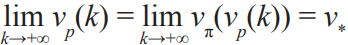. The ideal case is that for any k before reaching the optimum, we have α(k) > 0 (v_p(k) is monotonically increasing) and 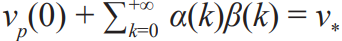. Certainly, other cases may appear in real applications. For example, there exist some k when α(k) < 0 or β(k) > 0, which lead to the interruption of the positive feedback. To ensure continuity of the positive feedback, theoretic support is needed, and adequate tuning of hyper-parameters is also required to fill the gap between theory and application.

On one hand, α(k) > 0 is ensured by the training of neural networks. For example, the loss function l = –π^T ( p(k))log p(k) and the gradient descent algorithm are applied to train neural networks. According to the Gibbs inequality [33], if and only if p(k) = π( p(k)), l reaches the minimum. Although we have a theoretical guarantee, α(k) is influenced by the structure of the neural networks and hyper-parameters in the gradient descent algorithm, which may not lead to p(k) = π(p(k)); that is, α(k) = 1. In real application, we only need to ensure α(k) > 0 by properly tuning the hyper-parameters.

On the other hand，β(k) > 0 is guaranteed by the CI algorithm. After the improvement of the earliest ant system [27] algorithm, many algorithms have the convergence proof. The graph-based ant system algorithm converges to the probability of the optimal action being 1 [32]. Two other frequently used algorithms, the ant colony system [25] and the max-min ant system [12], converge to the probability of the optimal action being greater than the lower bound [33]. MCTS improves from the earliest version to the version involving UCT. This includes the upper confidence bound (UCB) [34] for the selection and converges to the probability of the optimal action being 1 [30]. AlphaZero brings the predictor UCB (PUCB) algorithm into MCTS, and the PUCB algorithm alone without MCTS converges to the probability of the optimal action being greater than the lower bound [35]. Although this particular MCTS in AlphaZero does not have the theoretical proof, it can be seen from real applications that β(k) > 0 is ensured, and adequate tuning of hyper-parameters is required to fill the gap between the theory and application.

Under the condition that the perfect intelligence v* is finite, there are two types of intelligence convergence. One is that the individual intelligence approaches the same limit as the group intelligence. This means that either the perfect intelligence is already reached, that is, or the CI algorithm is not sufficient to produce higher group intelligence, that is, The other is that the individual intelligence approaches a limit that is lower than the group intelligence. This means that either the capacity of the individual intelligence is not sufficiently large, or the training method is no longer effective, that is, lim α(k) = 0 k→+∞ and

Compared with current machine learning methods, the CI evolution theory has some advantages. Deep learning is powerful but relies on an extremely large amount of high-quality labeled data, which is expensive. Reinforcement learning provides an evolution environment for the individual intelligence agent to evolve by inexpensive reward signals, but the learning efficiency is low because of the trial-and-error nature. The CI algorithm is able to make group intelligence emerge from nothing, but it lacks a mechanism to evolve individual intelligence. Combining the strengths of deep learning, reinforcement learning, and the CI algorithm, the CI evolution theory enables individual intelligence to evolve with high efficiency and low cost through CI emergence. Moreover, the evolution can start from ground zero, making the CI evolution theory a step further toward AGI.

《6 Applications in intelligent robots 》

6 Applications in intelligent robots

Traditional robots may utilize some computer vision or expert system technologies to realize certain kinds of intelligent behavior, but they lack the learning or evolving capability to automatically adapt to environment changes. For example, a welding robot is able to track the weld line through a 3D vision system and traditional feature-based vision algorithms. However, one has to adjust some critical parameters manually in a new welding environment to make the welding robot work properly. These manual efforts prevent the extensive applications of robots. Therefore, the robot industry demands intelligent robots that can automatically adapt to the environment like human beings

Our CI evolution theory has a natural application in intelligent robots, which is natively provided by a reinforcement learning environment through the closed loop of a sensor, intelligent agent, and actuator. An application of the theory is called the intelligent model. To facilitate the implementation of the intelligent model, a cloud-terminal platform was developed to create and evolve the intelligent models for intelligent robots.

Intelligent models for industrial applications are mainly divided into three categories: visual detection, data prediction, and parameter optimization. Among them, parameter optimization has the greatest demand. Therefore, an intelligent model for welding parameter optimization in a welding robot was implemented on the cloud-terminal platform.

With the development of science and technology in the field of steel welding, robotic welding has gradually replaced manual welding. During the welding process, the parameters of welding directly affect the quality of welding. Welding parameters include welding torch moving speed, current, voltage, welding torch angle, etc. Welding parameters need to be manually adjusted and optimized by welding engineers according to the conditions of the welding plate material, weld gap width, and thickness. In order to meet the needs of the intelligent application of welding robots in industry, we propose the technology of deep learning and reinforcement learning, combined with the 3D vision system of welding robots, to optimize welding parameters based on different welding conditions, i.e., generate a mapping relationship from the welding conditions to the optimal welding parameters. The welding robot could then automatically adjust the welding parameters according to the different welding conditions.

Considering the simplest welding scenario, the input feature only retains the weld gap width, which increases uniformly from zero. The output parameter only controls the moving speed of the welding torch.

The objective of the welding parameter optimization is to obtain the best welding quality. Specifically, for a smaller weld gap width, the solder width is expected to be kept at 5 mm; for a larger weld gap width, the solder width is expected to be 2 mm larger than the weld gap width. No matter how wide the weld gap is, the ideal solder height is 1 mm. Fig. 5 shows the relationship between the weld gap width and weld plate length. Fig. 6 shows the relationship between the ideal solder width and weld gap width.

《Fig.5》

Fig. 5. Relationship between the weld gap width and weld plate length.

《Fig.6》

Fig. 6. Relationship between the ideal solder width and weld gap width.

In the welding process of a weld gap, a small interval of a certain length is regarded as the welding point, starting from the beginning of the weld gap. The number of welding points is expressed by n. The gap width, solder width, and solder height of the welding point at each time step are expressed by g_i , w_i , and h_i , respectively. The time step of the i-th welding point is expressed by t_i . We define the simplified Markov decision process model as follows. Assuming that the environmental state s_t =g_i at time step t, then the action of the agent at time step t is the moving speed v_ti of the welding torch at the i-th welding point denoted by a_t = v_ti. Assuming that the discount factor is zero (only considering the immediate reward), then the difference between the actual welding effect and the ideal welding effect for every welding point is taken as a reward for this moment.

Fig. 7 shows the training flow chart of the welding parameter optimization intelligent model. To train this intelligent model, we first go to the welding site to collect actual welding effect data. Then, we train the value network offline. Finally, we use this value network to train the policy network (welding agent). Fig. 8 shows the relationship between the speed of the welding torch and the width of the weld gap.

《Fig.7》

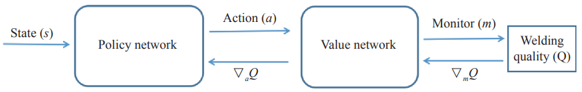
Fig. 7. Training flow chart of the welding parameter optimization intelligent model.

《Fig.8》

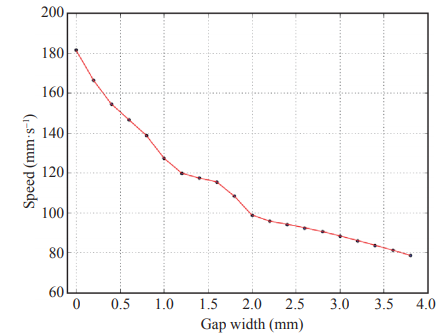
Fig. 8. Policy network, i.e., the relationship between the speed of the welding torch and the width of the weld gap.

We deployed this intelligent model on the cloud-terminal platform and tested it on the welding site (Fig. 9). The model achieved good welding quality. It can be seen that the policy network we obtained for the linear widened straight weld gap basically meets the requirements.

《Fig.9》

Fig. 9. On-site welding test.

For simple welding scenarios, single agent offline reinforcement learning can achieve a relatively high level of intelligence, i.e., welding quality. If the welding conditions are complex, it is necessary to perform an online welding quality assessment first and then carry out online intelligent evolution according to the theory of CI evolution. This will achieve a higher level of intelligence.

《7 Conclusion 》

7 Conclusion

CI emergence and deep neural network evolution are the key factors that have allowed the AlphaZero program to reach superhuman performance in a number of games. To combine CI with deep learning and reinforcement learning, a general theory of CI evolution has been presented. A demo application of this theory in a welding robot has also been discussed. As the proposed theory is a general framework toward AGI, we look forward to using it in more applications in the future.