《1.Introduction》

1.Introduction

Computing and implementing an optimal  production  schedule can reduce  operational  costs,  increase  profit  margins,  and  avoid deviations from environmental constraints [1]. However, complex industrial plants can have multiple production, storage, and distribution subsystems, several distinct raw materials and intermediate and final products, and intricate connections between all these elements that make scheduling a difficult decision-making process.

Scheduling problems typically deal with four main decisions [1]:① determining the required tasks to fulfill the corresponding objectives, requirements, and/or demand targets; ② assigning each task to a processing unit or resource that is available in the network; ③ defining the sequence in which the tasks will be executed; and ④ timing the tasks—that is, determining when to start and stop each one (Fig. 1). Optimal scheduling decisions are those that maximize or minimize a desired objective such as profit, total cost, lead time, and so forth. Scheduling software and tools based on mathematical programming is becoming more usual in practice.

《Fig. 1》

Fig. 1. Main scheduling decisions.

The scheduling of gasoline-blending operations is an important and relevant industrial problem because gasoline accounts for 60%– 70% of the total profit of an oil refinery [2–4]. In a gasoline-blending system, components from dedicated supply tanks are mixed in blending tanks or in-line blenders and sent to product tanks. Blending tanks can either have flow in or out (Fig. 2), resembling batch operation. In contrast, in-line blenders operate in a continuous manner (Fig. 3). In addition to the four decisions mentioned earlier, scheduling blend operations should also involve determining the blend recipes—that is, the amounts of components to mix such that products’ quality properties meet given specifications.

The gasoline-blending system studied in this work is described in Fig. 3. Gasoline blending is carried out by one or more continuous blenders. Each blender is connected to the sources of blend components. Blended material in some refinery configurations goes to a storage tank, while in other configurations, it can go directly to the pipeline. Since there are several grades of gasoline produced (e.g., regular, medium, premium), the blender switches  from  blending one grade to another. Each switch requires (partial) realignment of blend feeding lines, which leads to a loss of blending capacity. In addition, switching to a different range of quality properties often requires resetting or recalibration of the analyzers used to measure them.

《Fig. 2》

Fig. 2. Batch-blending system. The variable t means time period.

《Fig. 3》

Fig. 3. General scheme of the continuous gasoline-blending system studied in this work.

Some of the most important quality properties of gasoline are research octane number (RON), motor octane number (MON), Reid vapor pressure (RVP), density, sulfur, aromatics (Ar), and olefins (Ol) content. RON, MON, and RVP do not blend linearly; thus, considering nonlinear blending rules for such quality properties in the scheduling model can increase the accuracy of  the solution and reduce quality giveaways [4,5].

Since the 1960s, there has been a significant effort to derive so called “blend indices.” These are nonlinear transformations of the actual quality properties of the blend components, which then, as a linear combination, can predict the quality of the blend. Even with this approach, two issues remain:

(1)If a product is blended into a tank, there is always some material in the tank (the so-called “tank heel”) left over from previous blends. Any new blend must include the properties of the material in the tank in the calculation of the new blend recipe, which leads to a nonlinear blending model for multi-period scheduling, even when using blend indices.

(2)Blend properties calculated from these indices are not 100% accurate, and a cumulative annual quality giveaway of, for example, octane can amount to very large cost increments. This forces the use of nonlinear blending models for the calculation of, for example, octane numbers.

Mathematical models  for scheduling  problems are  usually  formulated as mixed-integer linear programming (MILP). However, for gasoline blending, nonlinear behavior is intrinsic to the corresponding process and mixed-integer nonlinear programming (MINLP) needs to be employed for the sake of accuracy. Most nonlinear terms are non-convex, making convex optimization techniques ineffective. A global optimization approach is thus required. Before describing the proposed global optimization method, a brief review of previous work is presented in the following paragraphs.

《1.1. Literature review on refinery scheduling》

1.1. Literature review on refinery scheduling

Scheduling models can be divided into two main categories based on the treatment of the time domain: discrete and continuous time formulations. In discrete-time models, the time horizon is divided into several time periods of known duration with fixed start and end time. In continuous-time models, the time horizon is partitioned into time slots whose duration will be determined by the optimization. While continuous-time models generate problems with fewer discrete variables than their discrete counterparts, they are more complex to formulate and often feature many “big-M” constraints that, due to their weak relaxations [6], compromise computational performance. More in-depth reviews of scheduling formulations can be found in Refs. [1,7–9].

Gasoline blending has been studied by many researchers due to its commercial importance and non-convex features, which makes it a suitable subject for testing different formulations and algorithmic approaches. Operational constraints found in gasoline blending are related to the presence of multipurpose tanks and non-identical blenders, to different storage-tank policies (e.g., whether the simultaneous receipt and delivery of material is allowed or not), and to practical aspects such as minimum blend sizes and minimum blender running and setup times. Not all of these constraints are considered in published scheduling models. In some cases, blend recipes are assumed to be fixed (i.e., they cannot be optimized). The downstream distribution or shipping problem (i.e., timing delivery tasks to fulfill the demand) is sometimes also part of the blend-scheduling problem.

Méndez et al. [2] presented both a discrete and continuous-time MILP model to schedule gasoline-blending operations. An iterative method was employed to handle nonlinear blending rules while preserving the linearity of the models. Several key operational constraints were omitted and the distribution problem was not considered.

Jia and Ierapetritou [10] developed a continuous-time MILP model to simultaneously schedule gasoline-blending tasks and distribution operations. The linearity of the model was maintained by using given preferred recipes. Their model was later extended to schedule operations of the main processing units in an oil refinery [11].

Glismann and Gruhn [12] used a two-level approach based on discrete-time models. Blend recipes and production targets were computed first using a nonlinear programming (NLP) model. Then a MILP model was employed to solve the short-term scheduling problem using such recipes and targets. The scheduling model was based on the resource-task-network (RTN) representation and did not consider multipurpose tanks or the delivery-scheduling problem.

Li et al. [13] formulated a continuous-time MILP model featuring a common time grid for all units (i.e., blenders and tanks). Li and Karimi [3] extended and improved this MILP model by using unit specific time grids and including most of the operational constraints found in practice. Both models optimized blend recipes using blend indices. Based on these two previous works, Li et al. [4] presented a unit-specific continuous-time MINLP formulation where nonlinear terms arise from enforcing constant blending rates.

Castillo and Mahalec [14] developed a three-level decomposition algorithm through which recipe optimization can be done using linear and/or nonlinear blending rules. They considered the distribution problem, blend-size threshold constraints, parallel non-identical blenders, swing tanks, and product-dependent setup times. A discrete-time model was formulated for each level. The first level optimized the blend recipes, the second level approximated the production schedule, and the third level computed a detailed blend-and-delivery schedule. Due to the large size of the scheduling model at the third level for the entire horizon, it was solved in subintervals. Solutions computed by this approach were better and the execution times for large problems were two orders of magnitude shorter than those from previous methods [3,13]. In their subsequent work, Castillo and Mahalec [15] introduced a significantly modified version of the continuous-time scheduling model from Li and Karimi [3] (with a smaller number of binary variables [16]) for dealing with the third level. Case studies with nonlinear blend-scheduling problems were solved very close to global optimality with short execution times.

Lotero et al. [17] proposed another formulation of the multi-period pooling problem. They denominated this discrete-time MINLP formulation as a hybrid of a source-based model (similar to Castro’s split-fraction model [18]) and a concentration-based model [19]. Redundant constraints were added to improve the linear relaxation, and the model was solved using a two-stage MILP-NLP approach. The MILP was a relaxation of the original MINLP model. The NLP model was obtained by fixing the integer variables of the original model to the values computed by the MILP. The algorithm adds integer, optimality, or feasibility cuts to the MILP model at each iteration, and stops when the difference between the MILP and NLP solutions is smaller than a pre-specified tolerance.

Cerdá et al. [20] presented a continuous-time MILP formulation that uses floating slots dynamically allocated to time periods while solving the problem. The model included most of the operational constraints found in practice. Cerdá et al. [21] then extended the model to handle nonlinear blending rules, thus formulating a continuous-time MINLP model. An approximate MILP formulation was derived by replacing the nonlinear blending rules with linear blend indices. The values of the binary variables computed by this MILP were fixed in the original MINLP, thus becoming an NLP that was solved to find a near-optimal solution of the original problem.

《1.2. Literature review on global optimization》

1.2. Literature review on global optimization

Global optimization of nonlinear non-convex problems has been a subject of extensive research over the last three decades. Even though powerful commercial solvers have been developed [22,23], there has been a continuous stream of advances in the field.

Global optimization algorithms have in common  the  generation of a convex relaxation of the problem, which provides a lower bound to the value of the objective function, and a way to generate feasible solutions (the upper bound). In addition, they have a method of bringing the lower and upper bounds together, so that the optimality gap can be reduced to ε-tolerance.

Computing a tight lower bound is absolutely critical. This may involve replacing the original formulation with an equivalent that preserves the feasible space but has a stronger relaxation (the different formulations for the pooling problem are a well-known example [24]). Another option is to reorganize the model constraints and add others that, although redundant in the original space, strengthen the relaxation. This procedure is known as the reformulation linearization technique [25]. The disadvantage is that there is no systematic way of knowing where to act in order to move toward a stronger relaxation.

A widely used method that guarantees convergence to the global optimal solution is known as spatial branch-and-bound [26,27]. It is an essential element of commercial solvers such as BARON [22], ANTIGONE [23], Couenne [28], and SCIP [29]. Spatial branch-and bound works by iteratively reducing the domain of the variables, one by one, which in turn improves the quality of the convex relaxation. Note that if the initial relaxation is weak, due to the presence of many non-convex terms, convergence can be rather slow. It is thus important to have good branching strategies and bound-tightening techniques. Optimality-based bound tightening (OBBT) is an example of the latter. Although typically applied only at the root node or up to a limited depth [28], recent results have shown that applying OBBT in every node may lead to considerably lower optimality gaps [30]. OBBT involves solving one minimization and one maximization problem for each variable (appearing in non-convex terms) in order to generate tighter lower and upper bounds. It can be solved sequentially—which has the advantage of generating tighter variable bounds and the disadvantage of being computationally expensive when dealing with a large number of variables—or in parallel [31].

Bilinear terms are a common source of non-convexities in process systems engineering. They can be relaxed using the McCormick envelopes, considering either the full domain of the variables [32] or a reduced domain following partitioning [33,34]. Simultaneous domain partitioning involves adding a new set of binary variables to the problem and guarantees global optimality in the limit of an infinite number  of  partitions.  Spatial  branch-and-bound  can  thus be avoided. One critical aspect concerns the scaling of problem size with the number of partitions. Earlier piecewise relaxation techniques [33] scale linearly, while recent formulations scale logarithmically. Examples of the latter are described next.

Misener et  al.  [35]  developed  a  global  optimization  algorithm for the standard pooling problem and concluded that the logarithmic scheme is more advantageous for more than eight partitions. Kolodziej et al. [19] proposed a MINLP formulation for the multi-period pooling problem, in which nonlinearities arise from using the dynamic inventories of tanks as blend components. They employed a radix-based discretization technique that partitions one variable in every bilinear term to obtain a MILP relaxation. This discretization technique is known as multi-parametric disaggregation [36]. Castro [37] developed the normalized multi-parametric disaggregation technique (NMDT) [36], which works by discretizing the range between a variable’s lower and upper bounds (belonging to [0, 1]). The advantage is that the number of partitions becomes the same for every discretized variable, even if their domain is different (when using a global discretization level parameter). NMDT has been successfully used to solve multi-period blending problems to global optimality, both as a stand-alone approach [18,38,39] or integrated in a spatial branch-and-bound algorithm [30].

Overall, contributions from cited works have enabled optimal solutions of gasoline blend-scheduling problems up to a certain model size. However, when dealing with large-scale problems, the computation and validation of global optimal solutions remain a difficult  challenge.

《1.3. Contributions of this work》

1.3. Contributions of this work

This work presents a novel deterministic global optimization algorithm to solve non-convex MINLP or NLP models with nonlinearities that are strictly due to bilinear and/or quadratic terms. The main features of this algorithm are:

• The use of different linear and piecewise linear relaxation techniques to derive convex relaxations of the original non-convex model;

• The collection of  different feasible solutions from the convex relaxation, which provide starting points for a local nonlinear solver to find feasible solutions of the original model;

• A dynamic increase in the number of partitions for piecewise linear relaxations;

• The reduction of the domain of the variables involved in nonlinear terms by means of an OBBT method; and

• The parallelization of the steps regarding computation of feasible solutions and the OBBT method.

The algorithm is tested on different gasoline blend-scheduling examples. For this class of problems, the results show that the proposed algorithm is on par with or better than two leading commercial global solvers.

The rest of this paper is organized as follows: Section 2 describes the problem statement and the assumptions made. Section 3 reviews the scheduling model employed in this work and presents the nonlinear equations used for octane blending. Section 4 briefly explains the piecewise linear relaxations employed to compute the estimates of the global solution. Section 5 describes the OBBT method to reduce the domain of the variables involved in nonlinear terms. Section 6 presents the steps of the global optimization algorithm. Section 7 contains the data describing the test examples. Section 8 shows the results obtained with the proposed algorithm and provides a comparison with other methods. The paper ends with conclusions in Section 9.

《2. Problem statement》

2. Problem statement

Given a blending system (i.e., storage tanks, blenders, and their interconnections; see Fig. 3), a scheduling horizon, a set of blend components and their corresponding supply and quality profiles along the horizon, a set of products and their minimum and maximum quality property specifications, a set of delivery orders for each product, and the initial inventory levels, it is required to determine the blend recipes, the production and delivery sequences, and the inventory profiles of all tanks, while minimizing the cost of the blended materials plus the switching costs (i.e., number of blend runs, number of tanks delivering the same order, and product transitions in the swing tanks) and the demurrage costs (i.e., late deliveries).

The following constraints are considered:

(1)If a blender is to produce a product, it must blend at least a minimum  amount.

(2)A blender can produce at most one product at any time. Once it begins blending, it must operate for some minimum time before it can switch to another product.

(3A blender requires a minimum setup time during a product changeover.

(4)A blender can feed at most one product tank at any time (industrial practice).

(5)Product tanks can only store one product at any time.

(6)Product tanks cannot receive and deliver material at the same time.

The assumptions made in this work are:

(1)The flow rate profile of each component from the upstream process is piecewise constant.

(2)The component quality profile is piecewise constant.

(3)Perfect mixing occurs in each blender.

(4)There is only one tank for a given blend component.

(5)Only swing tanks can change their product service (i.e., change from storing one product to storing another).

(6)Changeover times between products are negligible for swing tanks.

(7)For each blender, changeover times between product blending are product dependent but sequence independent.

(8)Each order involves only one product (any original order involving different products can be disaggregated into orders of a single product).

(9)All orders are fulfilled during the scheduling horizon.

In summary, this problem considers the scheduling of blending and delivery operations, recipe determination, and product allocation of swing tanks along the scheduling horizon.

《3.Gasoline blend-scheduling model》

3.Gasoline blend-scheduling model

The scheduling model employed in this work is the one presented by Castillo and Mahalec [16]. It employs a continuous-time formulation, considers nonlinear blending equations, and does not allow simultaneous receipt and delivery by product tanks. This is a non-convex MINLP model, and it will be denoted as model P (or problem P). The main features of the scheduling model are highlighted in this section.

The scheduling model uses unit-specific time slots of varying length to determine when a specific task needs to be executed in each unit (blenders and tanks in this case). We assign a sufficiently high number of time slots, which will likely be higher than the number of slots required for blending each grade. This ensures that there are sufficient degrees of freedom (enough available switches) to meet the varying product-delivery schedule.

The start time of a unit slot is equal to the end time of the previous one. The first unit slot starts at the beginning of the scheduling horizon, and the end of the last unit slot matches exactly the end of the horizon. Blending tasks begin at the start of a time slot, but can finish before its end. Delivery tasks from product tanks can start and finish within the corresponding slot. It is assumed that component tanks are continuously receiving material at some specified rate (i.e., the supply profile). Time periods are used to delineate the points where changes occur in the supply rates and/or quality of blend components. Time slots are assigned to these time periods. A time slot must end within its assigned period. However, for component tanks, the last time slot of a period must end exactly at that period’s boundary (in order to properly respect the changes in supply rates and/or quality of blend components). Fig. 4 shows a graphical representation of these unit-specific time slots for a blending system with two blend component tanks (CT1, CT2), one blender (B1), and two product tanks (PT1, PT2). Unit slots 1 and 2 are pre-assigned to period 1, while slots 3 and 4 are pre-assigned to period 2. Note that the optimization has determined that slot 3 in the CT2 grid, and slot 4 in the PT1 grid, have zero length.

《Fig. 4》

Fig. 4. Representation of unit-specific time slots employed in the scheduling model.

The objective of the scheduling model is to minimize the blend cost (i.e., materials cost), the switching cost associated with each blend run, product changeovers in the swing tanks, the number of “delivery runs” (i.e., the number of time slots used to deliver a specific order from a given tank), and the demurrage cost. Delivery runs are penalized in order to avoid computing delivery schedules that deliver the same order from several tanks at the same time, and to minimize intermittent deliveries of the same order from the same tank.

Binary variables are employed in the model to determine, at each time slot, the following discrete decisions:

• Which product tank each blender is feeding (one variable for each blender-tank connection);

• What gasoline grade is stored in each product tank (one variable for each grade-tank pair); and

• What demand order each product tank is partially or completely fulfilling (one variable for each tank-order connection).

With these binary variables, other discrete decisions can be modeled with 0–1 continuous variables, such as:

• What gasoline grade each blender is producing;

• The status of a blender (running or idle);

• The transition of a blender from running to being idle, or vice versa;

• When a new blend run starts;

• Product transitions in the blenders; and

• Product changeovers in the swing tanks.

The  scheduling  model  also  considers  variable  blending  rates, variable delivery rates, blender and product-specific setup times for the blenders (i.e., idle times for, e.g., cleaning or sensor recalibration purposes), maximum delivery rates from blend component tanks to the blenders, minimum blend size, and minimum running times for each blender and product. Other constraints include the material balances, product composition specifications, product quality specifications, and linear and/or nonlinear blending equations.

The difficulty in solving this scheduling model to global optimality arises from the following factors:

• The significant number of discrete decisions that can be made, which are directly related to the number of time slots, gasoline grades, blenders, product tanks, and demand orders (the combinatorial nature of the problem);

• The inclusion of nonlinear blending equations (the non-convex nature of the problem); and

• All the considered operational constraints.

Castillo and Mahalec [16] found that introducing constraints regarding minimum blend cost and minimum switching cost can improve the quality of the solution and reduce the execution times for small to medium-size problems. The minimum blend cost is computed using the approach delineated in Castillo et al. [40].

The nonlinear blending equations are presented next, since they were rewritten in such a way that nonlinear terms are only bilinear or quadratic.

《Nonlinear blending equations》

Nonlinear blending equations

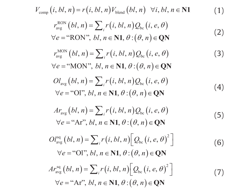
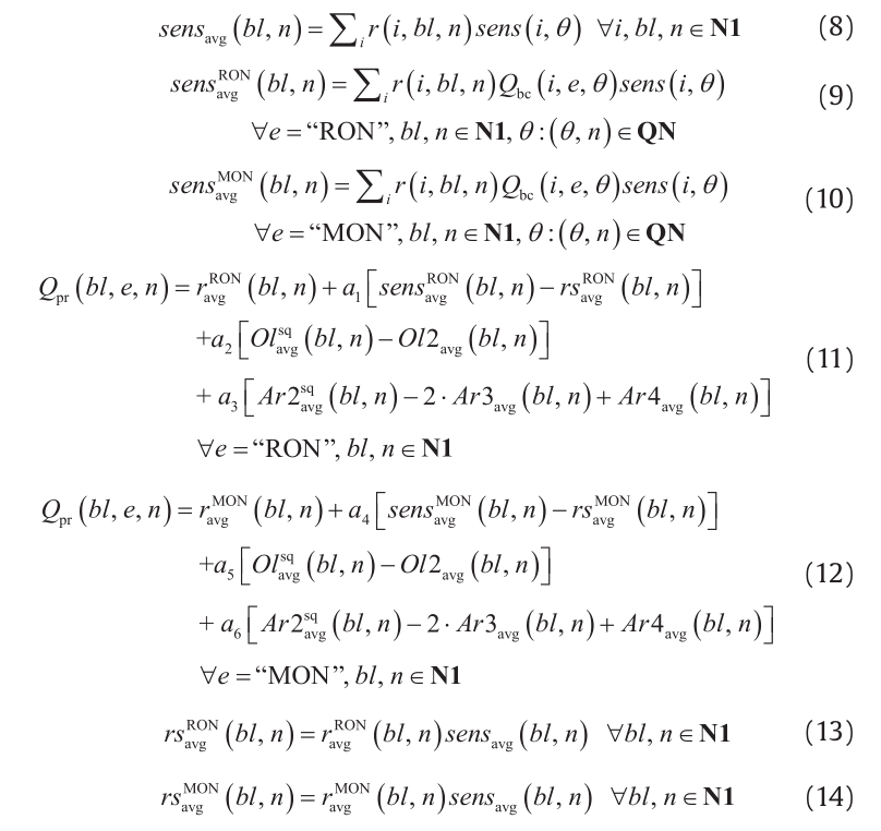
Eq. (1) to Eq. (19) are the proposed reformulation of the ethyl RT-70 model for octane blending [5,41]. Bilinear terms appear in Eqs. (1), (13), (14), and (18). Quadratic terms appear in Eqs. (15), (16), (17), and (19). Main sets, subscripts, variables, and parameters are described next. Set I = {i} consists of the blend components, BL = {bl} is constituted by the blenders, N1 = {n} is the time slots, and set QN = {(θ, n)} represents the time slots associated with each quality profile θ. Variable V_comp(i, bl, n) indicates the volume of blend component i to blender bl during slot n. Variable V_blend(bl, n) is the volume being processed by blender bl during slot n. The volume fraction of component i going into blender bl during slot n is denoted by variable r(i, bl, n). Parameter Q_bc(i, e, θ) represents the value of quality property e for blend component i and quality profile θ. _sens(i, θ) is a parameter known as the octane number sensitivity; it is the difference between the octane numbers, that is, RON – MON, of blend component i and quality profile θ. The values for the ethyl RT-70 model coefficients are taken from Singh et al. [5] and are as follows: a₁  = 0.03224, a₂  = 0.00101, a₃  = 0, a₄  = 0.0445, a₅  = 0.00081, and a₆ = −0.0645 × 10⁻⁴.

《4.Piecewise linear relaxations》

4.Piecewise linear relaxations

As mentioned in Section 1, the use of piecewise linear relaxations is becoming more widespread due to the maturity of MILP solvers. Piecewise McCormick relaxation (PMCR) and the NMDT will be employed in this work. These techniques replace each bilinear term in model P with a single variable, thus linearizing the corresponding equations. This single variable is then subject to various linear constraints, which add extra continuous and binary variables to the model. If equal to 1, these extra binary variables activate a specific interval of the domain (i.e., partition) of one of the variables in the bilinear term (denoted as the discretized variable). The number of partitions is denoted as NP, and it is assumed that all discretized variables have the same number of partitions. PMCR has a linear relation between NP and the number of extra binary variables required per discretized variable, while NMDT exhibits a logarithmic relation.  For  a  more  detailed  explanation  of  these  methods,  the reader is encouraged to review Refs. [16,37].

The resulting MILP model is denoted as model PR and is a relaxation of problem P. This means that the optimal solution of model PR is a valid estimate of the global solution of P (in the minimization case, this will be a lower bound, LB). Moreover, an estimate of the best possible solution of model PR is a valid estimate of the global optimum of P. Therefore, even if model PR is not solved to optimality by a MILP solver within a given allocated time, a new estimate of the global solution can still be found. The larger the number of partitions, the closer model PR is to model P; see Fig. 5 for  an  illustration  with  an  example  involving  a  single  discretized variable.

《Fig. 5》

Fig. 5. Accuracy of the relaxation (f0  ) with respect to exact representation (f0) of the boundaries of a feasible region increases with the number of partitions (maximization problem).  (a)  10  partitions;  (b)  100  partitions.

If  the relaxation is tight, then its optimal solution will be very close to the original optimum. Hence, a strategy to find a feasible solution to the original problem P (in the minimization case, this will be an upper bound, UB) is to initialize P with the optimal solution of model PR. Since some MILP solvers, such as CPLEX, can store multiple feasible solutions to the MILP problem, potentially leading to different solutions of P due to the different starting points, we use a multi-start strategy in parallel fashion. Note that, for practical reasons related to the speed and robustness of commercial solvers, it is more convenient to solve NLP models instead of MINLPs. This is the reason why the values of the binary variables are fixed, converting problem P (MINLP) into PF (NLP). The compact notations of models P,PR, and PF are as follows:

Model P:

Model PR:

Model PF:

Note that, in this section, set M = {m} represents all the original constraints, set N = {n} represents all the constraints required by the piecewise linear relaxation technique, and set BLT = {(i, j)} represents all the bilinear terms. Variables x and y are the original continuous and binary variables, respectively, and v and z are the extra  continuous  and  binary  variables,  respectively,  required  by the relaxation strategy. Variable w_ij  is the continuous variable that replaces the bilinear term x_i x_j. Scalars lx, ly, lw, lv, and lz represent the size of vectors x, y, w, v, and z, respectively. Parameters x^L and x^U are respectively the lower and upper bounds of the x variables. Note that quadratic terms can be treated as bilinear terms.

《5.Tightening bounds on the variables》

5.Tightening bounds on the variables

Model PR becomes tighter (i.e., closer to model P) as the number of partitions of the discretized variables is increased. However, an increase in the number of partitions produces an increment in the size of model PR and, after a certain number of partitions, model PR can become computationally intractable. Therefore, another technique is required in order to avoid the necessity of a large number of partitions. In this work, an OBBT method is employed [34,42]. The idea is to reduce the domain of the variables involved in nonlinear terms by computing new bounds of these variables by solving two optimization problems (a maximization problem and a minimization problem per variable). This is done after a new and better feasible solution to P is computed. After reducing the domain of the variables, model PR becomes closer to P without increasing the number of partitions, as shown in Fig. 6.

《Fig. 6》

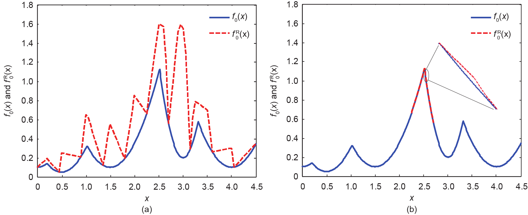
Fig. 6. Accuracy of the relaxation increases when the domain of the variables involved in nonlinear terms is reduced. (a) 10 partitions with x ∈ [0, 4.5]; (b) 10 partitions with x∈[2.25, 2.7].

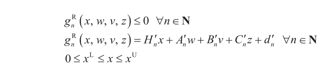
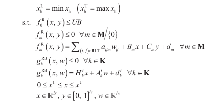
The mathematical model used in OBBT is denoted as model PRB, which is constructed as a relaxation of P, but with a different objective function and an extra constraint. To compute a lower bound of variable x_h , that is x^l_h , the objective function is to minimize this variable. To compute an upper bound of variable x_h , that is, x^u_h , the objective function is to maximize this variable. In order to compute new bounds, the extra constraint added imposes the condition that the value of the relaxed version of the original objective function, that is, f^R₀  (x, y), must be at least as good as the current best feasible solution.

Note that models PR and PRB can use different relaxations. In this work, model PRB employs standard McCormick envelopes [32] and integrality requirements on variables y are dropped, thus reducing PRB to linear programming (LP). The lower and upper bounds of variable xh are updated with the optimal solutions of the corresponding LP model. Compact notation of model PRB is shown below for a minimization problem.

Model PRB:

OBBT consists of solving these LP models for all the variables involved in nonlinear terms, in a parallel framework, to reduce execution times. Thus, the bounds will generally be weaker than when solving the problems sequentially. Since the number of instances to solve can be very large, instances are solved in different blocks. These blocks are defined by a maximum number of problems to be solved in parallel. After one block is solved, the corresponding bounds are updated and then the next block is solved. Fig. 7 shows the flowchart of the OBBT method. Note that OBBT is applied only once per variable.

《Fig. 7》

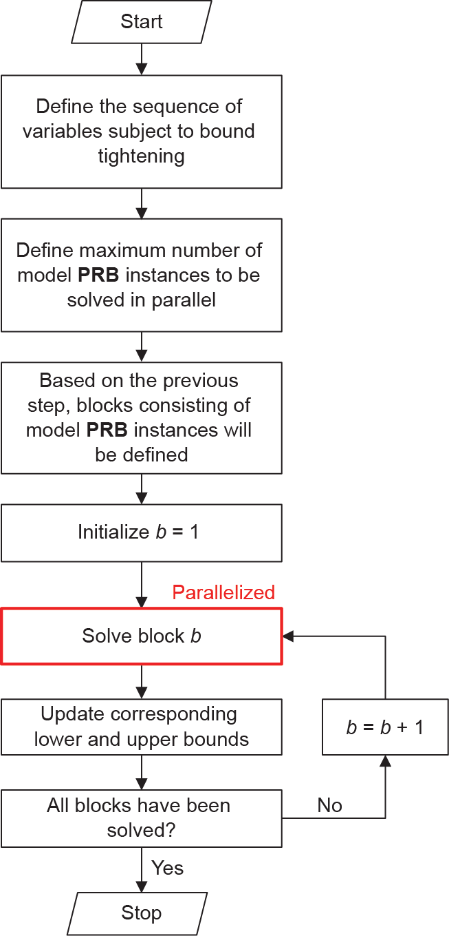
Fig. 7. Flowchart of the OBBT method. 

《6.Global   optimization  algorithm》

6.Global   optimization  algorithm

The steps  of the proposed  global  optimization  algorithm are presented next for a minimization problem. Fig. 8 shows the corresponding flowchart. Note that the algorithm can be applied to any MINLP problem with nonlinearities exclusive to bilinear or quadratic terms.

《Fig. 8》

Fig. 8. Flowchart of the global optimization algorithm.

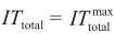
（1）Initialize algorithm parameters. Define the number of partitions to be used {NP₁, NP₂, …, NP_last} and set NP = NP₁. Set the lower bound LB = −∞, upper bound UB = +∞, total number of iterations counter IT_total = 1, iterations with the same number of partitions IT_sameNP = 1, maximum number of total iterations ,maximum number of iterations with the same number of partitions  , maximum total time , and minimum relative tolerance ε.

（2）Lower bound computation. Solve MILP model PR using the CPLEX solver with parallel and solution pool options active. Update LB with the best possible solution from CPLEX, if this value is greater than the previous LB.

（3）Upper bound computation. Use the solutions stored in the CPLEX solution pool as starting points for NLP model PF. Solve NLP model PF instances in parallel using a local nonlinear solver. Update UB if any of the computed solutions is feasible and has a smaller objective function value than the previous UB.

（4）Update optimality gap. The following formula is used in this step: Opt Gap = (UB – LB)/LB × 100

（5）​​​​​​​​​​​​​​Check termination criteria. Stop if Opt Gap ≤ ε, if if the total execution time is equal to or greater than , or if the number of partitions has already reached NP_last. Otherwise, continue to Step 6. 

（6）If the upper bound UB did not improve in Step 3, or if IT_sameNP= continue to Step 7. Otherwise, reduce the domain of the variables involved in nonlinear terms using the OBBT method described in Section 5; set IT_total = IT_total + 1 and  IT_sameNP= ITs_ameNP + 1, and then go back to Step 2.

（7）Increase the number of partitions to the next specified value. Set IT_total = IT_total + 1 and go back to Step 2.

Although the main elements of the algorithm have already been proposed (e.g., PMCR, NMDT, OBBT), the novelty is related to the way in which they are implemented. More specifically: ① the CPLEX solution pool is used to store starting points for model PF, ② instances of model PF are solved in parallel, ③ OBBT is applied to blocks of variables and in a parallel framework, and ④ no branching strategy is employed.

《​​​​​​​7.Case studies》

7.Case studies

The tests in this paper consist of Examples 4, 8, 12, and 14 from Li and Karimi [3]. The difference in this work is that the ethyl RT70 models are considered for blending RON and MON properties (as described in Section 3.1) instead of blend indices. RON index correlations from Li et al. [13], shown in Eq. (20) and Eq. (21), were used to compute the actual RON values from the blend indices given by Li and Karimi [3]. RBN denotes the research octane number blend index. MON values were assumed in this work and the corresponding minimum product specifications were set equal to zero; therefore, MON constraints will not be active at the optimal solution. Quality properties of blend components are assumed to be known (recall Section 2); therefore, Eq. (20) and Eq. (21) are only used to convert the blend components’ RBN values to RON values before the optimization runs (i.e., they do not appear in the optimization problems).

RBN = RON + 11.5  0 ≤ RON≤ 85                               (20)

RBN = exp (0.0135RON + 3.422042) RON > 85        (21)

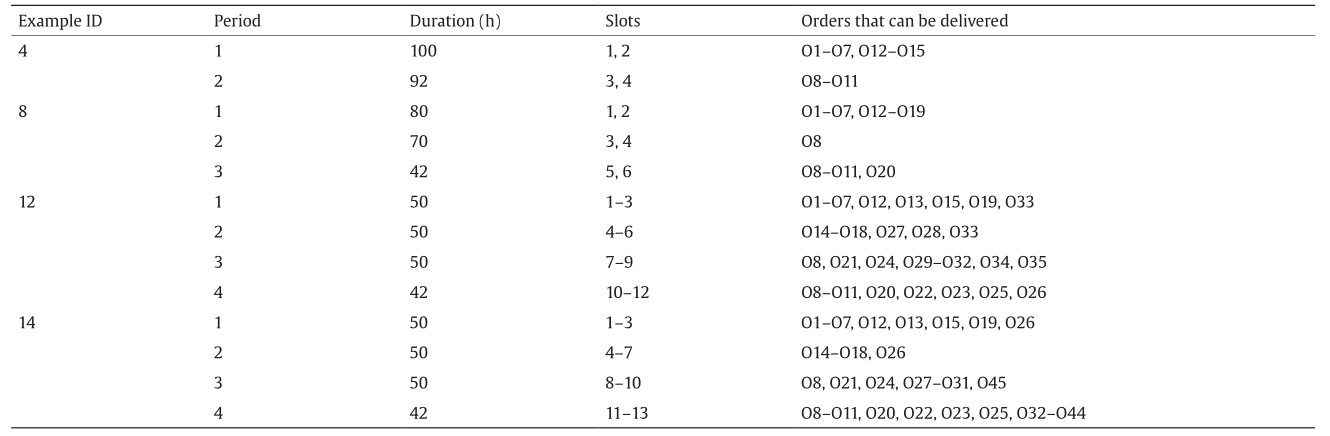
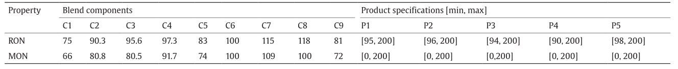
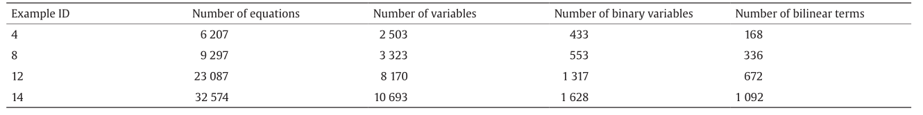
Table 1 describes the size of the blending system examples. Information about the periods, their duration, their corresponding time slots, and the orders that can be delivered within such periods is presented in Table 2. RON and MON values and their respective specifications are shown in Table 3. Table 4 presents the statistics regarding the size of model P when not using the constraints on the minimum blend and switching costs. When using such constraints, four equations are added to the model (minimum blend cost, minimum number of delivery runs, minimum number of blend runs, and minimum number of product changeovers in the swing tanks). Note that the size of the blending system and its corresponding scheduling model increase from Example 4 to Example 14.

《Table 1》

Table 1 Summary of the blending system examples.

《Table 2》

Table 2 Periods, duration, time slots, and orders that can be delivered in each period.

《Table 3》

Table 3 RON and MON values and specifications.

《Table 4》

Table 4 Statistics of model P.

《​​​​​​​8.Results》

8.Results

All the examples were solved on a computing machine Intel^® Core™ i7-4710HQ central processing unit (CPU), 2.50 GHz, 12 GB random-access memory (RAM), Windows 10 (8-core). The global optimization algorithm was implemented in Python 2.7. The Python script generates general algebraic modeling system (GAMS) files with the corresponding mathematical models, which are then solved by employing the GAMS-Python application program interface (API). The selected solvers were CPLEX 12.6 for model PR and model PRB, and CONOPT 3 for model PF.

The global optimization algorithm termination criteria were as follows: 0.01% optimality gap or 3600 s (1 h). There was no limit on the total number of iterations, nor on the iterations with the same number of partitions. The numbers of partitions in model PR when using PMCR were {2, 4, 8, 16, 32}, and when using NMDT were {10,100, 1000}.

The termination criteria for the MILP problems (instances of model PR) were: an optimality gap of 0.01% or 600 s. The CPLEX parallel option was active (in deterministic mode) with a maximum number of threads equal to 8. In addition, the CPLEX solution pool option was active with a maximum pool capacity of 30 and the replacement option that generates diverse solutions. Thus, a maximum of 30 instances of model PF was solved per iteration using the GAMS parallel computing grid facility. CONOPT 3 default termination criteria were used.

The termination criteria for the LP problems (instances of model PRB) were: optimality or 60 s. A maximum number of 100 LP problems were solved in parallel using the GAMS parallel computing grid facility.

For comparison purposes, the global commercial solvers BARON 15.9[33] and ANTIGONE 1.1 [34] were employed to solve the original model P using the same termination criteria as the proposed global optimization algorithm.

Section 8.1 presents the results obtained when not including the constraints on the minimum blend cost  and  minimum  switching cost, while Section 8.2 shows the results when such constraints are added to the model. A comparison with previously published heuristic methods is included in Section 8.3.

《8.1. Not using constraints on the minimum blend and switching costs》

8.1. Not using constraints on the minimum blend and switching costs

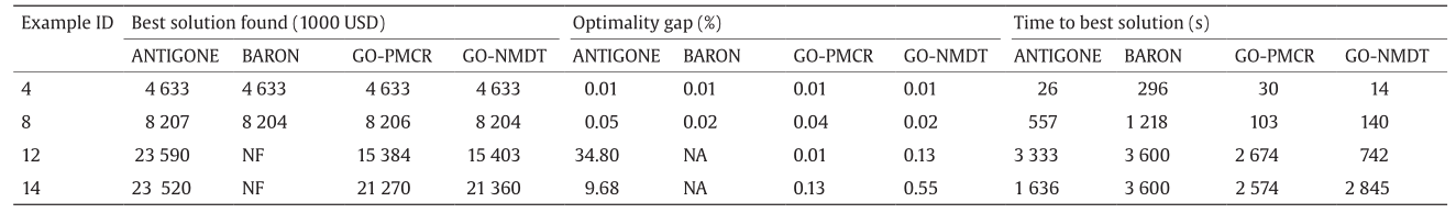
A comparison of the results obtained by the proposed algorithm with those obtained by commercial solvers is presented in Table 5. For simplicity, we refer to our proposed algorithm as GO-PMCR when it uses piecewise McCormick  relaxation  to  construct  model PR and as GO-NMDT when it employs the NMDT.

《Table 5》

Table 5 Summary of results (not using constraints on the minimum blend and switching costs).

ANTIGONE, BARON, and GO-PMCR compute the same solution for Examples 4 and 8. GO-NMDT computes the same solution for Example 4, but the final solution for Example 8 is slightly higher. GO-PMCR computes better solutions than GO-NMDT and ANTIGONE in all examples. In this work, this is because GO-PMCR can use more distinct numbers of partitions (2, 4, 8, 16, 32) than GO-NMDT (10, 100, 1000); thus, it generates more feasible solutions from the MILP relaxation.

BARON does not find a feasible solution for Examples 12 and 14 within 1 h. Based on the log files generated by commercial solvers, it seems that BARON relies more on the branching procedure, while ANTIGONE focuses more on the MILP relaxation and bound-tightening steps (as our proposed algorithm does). Feasible integer solutions for scheduling problems may be found only at deep nodes in the branch-and-bound tree [43], which can be of significant size when the number of binary variables is large.

In Examples 4 and 8, the algorithm and the commercial solvers compute similar optimality gaps. For Examples 12 and 14, BARON cannot compute an optimality gap (no feasible solution was found), and GO-PMCR obtains a lower optimality gap than GO-NMDT and ANTIGONE.

Both commercial solvers and the proposed algorithm did not solve all four examples to the desired tolerance within 1 h. The times reported in Table 5 are the times in which the best solution was found. GO-PMCR and GO-NMDT require shorter times than both commercial solvers. GO-NMDT is significantly faster than GO-PMCR only in the small-sized  Example 4. Note  that, for the number  of partitions selected, the size of the MILP relaxation grows faster with GO-NMDT than with GO-PMCR. Therefore, MILP relaxations are often faster to solve to optimality with GO-PMCR. However, GO-PMCR will require more iterations. Based on the three factors considered (i.e., best solution found, optimality gap, and time to best solution), GO-PMCR shows the best performance. Fig. 9 shows the total number of binary variables in the relaxation of the scheduling model (i.e., model PR) when using PMCR and NMDT, at each iteration of the algorithm and for each example. It shows that, for the selected partition values, PMCR requires fewer binary variables in the first 4–5 iterations than NMDT at any iteration. This is expected since the partitions when using PMCR are fewer than 8 in those iterations, and NMDT starts with 10. Note that flat sections in the curves indicate that the OBBT method was applied instead of increasing the number of partitions.

《Fig. 9》

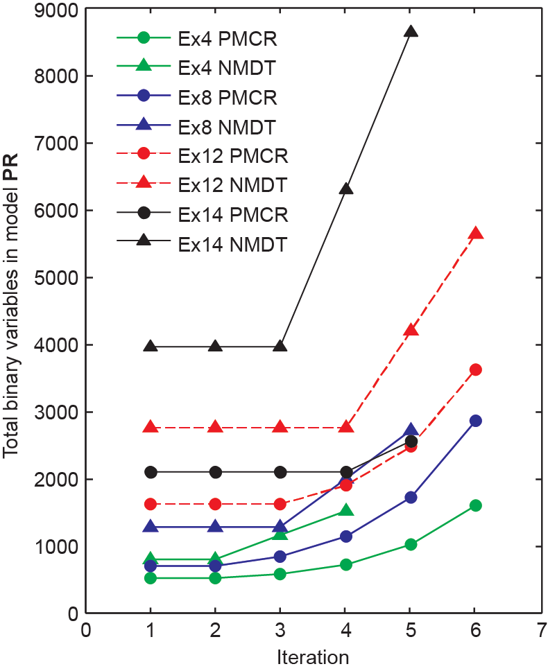
Fig. 9. Number of binary variables in model PR at each iteration of the algorithm.

The major differences between the proposed algorithm and BARON are:

• The use of piecewise relaxation methods for bilinear terms instead of standard McCormick envelopes; and

• Dynamically increasing the number of partitions in order to tighten the MILP relaxation, instead of implementing a branching strategy.

• These features seem to be adequate for the scheduling problems presented here. We do not claim that our proposed algorithm will always be better than BARON when solving a different type of problem.

Our proposed algorithm and ANTIGONE perform similarly, but differ mainly in the following areas:

• The use of NMDT as a piecewise relaxation technique;

• The use of the CPLEX solution pool to store feasible solutions from the MILP relaxations and use them as starting points to solve the NLP problem.

• When and how to apply OBBT; and

• How the number of partitions is increased in each iteration;

Finally, ANTIGONE and BARON can handle more than just bilinear and quadratic terms; in addition, they apply other mathematical techniques capable of improving performance (e.g., reformulationlinearization technique, cutting planes, feasibility-based bound tightening, different branching strategies, etc.).

NF = not found; NA = not available.

《8.2.Using constraints on the minimum blend and switching costs》

8.2.Using constraints on the minimum blend and switching costs

For this case, the results computed by the algorithm and commercial solvers are presented in Table 6. The most notable differences with respect to Table 5 are the smaller optimality gaps and the shorter times for Examples 4 and 8.

《Table 6》

Table 6 Summary of results (using constraints on the minimum blend and switching costs).

NF = not found; NA = not available.

Both commercial solvers and the algorithm find similar solutions for Examples 4 and 8. BARON still does not find a feasible solution for Examples 12 and 14 within the allocated time. GO-PMCR computes better solutions than GO-NMDT for Examples 12 and 14, which in turn has better solutions than ANTIGONE. Note that the addition of bounds caused an increment in the number of solutions for Example 8. Since the solutions from Section 8.1 are still feasible even with the inclusion of the constraints regarding minimum blend and switching costs, this suggests that such constraints are affecting the solvers. This effect is also observed in ANTIGONE in Examples 12 and 14.

Regarding optimality gaps, most of the same observations as in Section 8.1 can be made. Similar optimality gaps are computed by all methods for Examples 4 and 8. For Examples 12 and 14, GO-PMCR calculates lower optimality gaps than GO-NMDT and ANTIGONE.

Both commercial solvers and the proposed algorithm solve Example 4 to the desired tolerance; BARON is the slowest. For Example 12, the time to the best solution required by GO-PMCR is larger than that required  by GO-NMDT;  however,  it must  be considered  that GO-PMCR computes a better solution.

Overall, GO-PMCR shows the best performance once again. For illustration purposes, the blend and delivery schedules computed for Example 14 by the algorithm using PMCR are shown in Fig. 10 and Fig. 11, respectively.

《Fig. 10》

Fig. 10. Blend schedule computed for Example 14 by the proposed algorithm using PMCR. Kbbl is short for kilobarrel, 1 kbbl = 158.9873 m³.

《Fig. 11》

Fig. 11. Delivery schedule computed for Example 14 by the proposed algorithm using PMCR.

《8.3.Comparison with heuristic methods》

8.3.Comparison with heuristic methods

In this section, the proposed algorithm is compared with previously published heuristic methods [15,21]. Table 7 [15,21] contains the best solution found by those methods and the time required to compute such solutions. Note that heuristic methods do not compute an optimality gap since they aim to find close-to-optimal solutions very rapidly, and they do not spend time estimating and refining the value of the global optimal solution. These heuristic methods are tailored to the examples used in this work. These methods construct the final solution by decomposing the original problem into different levels, each one with different accuracy and complexity. Short execution times are achieved by solving the least complex level first and then, in each subsequent level, fixing the values of the most important variables to those from the previous level’s solution.

《Table 7》

Table 7 Comparison with heuristic methods.

​​​​​​​

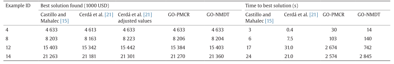
The objective function of the scheduling model employed in this work is the same as the one used by Castillo and Mahalec [15]. This objective function penalizes each individual blend run, even when the same product is being blended in contiguous blend runs. On the other hand, Cerdá et al. [21] did not penalize the number of individual blend runs, but only penalized the product transitions in the blenders. We show the adjusted values of the solutions reported by Cerdá et al. [21]; that is, individual blend runs are penalized.

All methods find the same solution for Example 4. In general, all the methods compute very similar solutions for the remaining examples. Solutions from Cerdá et al. [21] have higher costs for Examples 8, 12, and 14 because they did not originally penalize individual blend runs. The method from Cerdá et al. [21] might compute similar solutions to those from the other methods if it used the same objective  function.

Heuristic methods still require smaller execution times than the proposed global optimization algorithm. This is expected, because those methods do not involve as many steps as global optimization techniques. The proposed global optimization algorithm does not find solutions of the same quality as quickly as the two selected heuristic methods. To compute feasible solutions in each iteration, our proposed algorithm needs to first solve a MILP (i.e., model PR). The solution of the MILP is the most time-consuming step, thus reducing the speed required to compute new feasible solutions. Moreover, the small number of partitions at the beginning of the algorithm may result in weak MILP relaxations, which generate starting points for the NLP models that are far from the global optimum.

These results indicate the need to improve the corresponding step to compute feasible solutions, or to simply integrate heuristic methods into the proposed algorithm.

《​​​​​​​9.Conclusions》

9.Conclusions

In this work, we presented a global optimization algorithm that  can solve MINLP problems with bilinear and quadratic terms. The algorithm computes estimates of the global solution by constructing and solving MILP problems that are relaxations of the original problem obtained by using either PMCR or NMDT. These methods discretize the domain of one of the variables of a bilinear term into several partitions, and introduce extra binary and continuous variables into the  model.  To  improve  the  estimates  of  the  global  optimum,  the number of partitions is increased during the algorithm.

To avoid a rapid increase in the model size due to a large number of partitions, an OBBT method is used. The MILP relaxation will be closer to the original problem if the number of partitions stays the same but the domain of the variables is reduced. The OBBT method solves several LPs in a parallel setting.

The CPLEX solution pool is active and stores different feasible solutions found during the branch-and-bound procedure to solve the MILP relaxation. These solutions are then used as starting points for a nonlinear solver to find feasible solutions to the original problem. This step is also parallelized.

We showed that the proposed algorithm can be used to schedule gasoline-blending operations, taking into consideration the distribution problem and the most important operational constraints. We employ a continuous-time MINLP scheduling model [16] where the ethyl RT-70 models are used for octane blending.

The proposed algorithm was compared with two commercial solvers and two heuristic methods. The elements under evaluation were: the  best  solution  found,  the  corresponding  optimality gap, and the time to best solution. The proposed algorithm with PMCR showed a better performance than with NMDT. In our large-sized examples, the proposed algorithm with either PMCR or NMDT performed better than the commercial global solvers. This result shows that further research on this algorithm may be very promising. Both selected heuristic methods provided good solutions in shorter execution times than the global algorithms. This result indicates that the step to compute feasible solutions can still be improved.

We tested the performance of the algorithm by solving the scheduling model for two scenarios: ① not including lower bounds on the blend cost and switching costs, and ② including such bounds. The first problem is harder to solve and is representative of a kind of model one may write without diligently trying to reduce the search space as much as possible. Adding a tight lower bound to the blending cost as a constraint, as well as adding the lower bound to the switching costs, enables algorithms to search smaller spaces and improves their performance. This result also indicates that the relaxations are still not tight enough. Future work will include the derivation and addition of redundant and symmetry-breaking constraints; the testing of a different relaxation scheme for quadratic, cubic, and higher order terms (e.g., outer approximation); and the modification of the bound-tightening method in order to speed up the algorithm.

《​​​​​​​Acknowledgements》

Acknowledgements

Support by Ontario Research Foundation, McMaster Advanced Control Consortium, and Fundação para a Ciência e Tecnologia (Investigador FCT 2013 program and project UID/MAT/04561/2013) is gratefully  acknowledged.

《Compliance with ethics guidelines》

Compliance with ethics guidelines

Pedro A. Castillo Castillo, Pedro M. Castro, and Vladimir Mahalec declare that they have no conflict of interest or financial conflicts to disclose.

《Nomenclature》

Nomenclature

Sets and subscripts

BL = {bl}                   Blenders

E = {e}                      Quality properties

I = {i}                        Blend components and corresponding storage tanks

N1 = {n}                   Time slots

QN = {(θ, n)}            Time slot n is associated with the period with quality profile θ

Parameters

a₁, a₂, ..., a₆              Coefficients for the ethyl RT-70 model

Q_bc (i, e, θ)              Value of quality property e of blend component i during quality profile θ

sens (i, θ)                Octane number sensitivity, i.e., octane difference RONMON for blend component i during quality profile θ

Continuous variables

Ar_avg (bl, n)            Volumetric average of the aromatics content of the processed material by blender bl during slot n

Ar ^sq_avg (bl, n)        Volumetric average of the squared value of the aromatics content of the processed material by blender bl during slot n

Ar2_avg (bl, n)          Squared value of Ar_avg (bl, n) 

Ar2^sq_avg   (bl, n)    Squared value of Ar^sq_avg   (bl, n)

Ar3_avg (bl, n)         Product of Ar^sq_avg (bl, n) and Ar2_avg (bl, n)

Ar4_avg (bl, n)         Squared value of Ar2_avg (bl, n)

Ol_avg (bl, n)           Volumetric average of the olefins content of the processed material by blender bl during slot n

Ol ^sq_avg (bl, n)      Volumetric average of the squared value of the olefins content of the processed material by blender bl during slot n

Ol2_avg   (bl, n)      Squared value of Ol^sq_avg   (bl, n)

Q_pr (bl, e, n)         Value of quality property e of the processed material by blender bl during slot n

r (i, bl, n)              Volume  fraction  of  blend  component  i  going  into blender bl during slot n

(bl, n)            Volumetric average of the motor octane number of the processed material by blender bl during slot n

(bl, n)           Volumetric average of the research octane number of the processed material by blender bl during slot n

(bl, n)          Product of (bl, n) and sens_avg (bl, n)

(bl, n)          Product of  (bl, n) and sens_avg (bl, n)

sens_avg (bl, n)      Volumetric average of the octane number sensitivity of the processed material by blender bl during slot n

 (bl, n)         Volumetric average of the octane number sensitivity times the motor octane number

 (bl, n)        Volumetric average of the octane number sensitivity times the research octane number

V_blend (bl, n)       Volume being processed by blender bl during slot n 

V_comp (i, bl, n)    Volume of blend component i transferred to blender bl during slot n