
《 1.Introduction》
1.Introduction
Wind energy has emerged as one of the leading renewable sources of carbon-free electrical power production. Technological advancements and manufacturing innovations have successfully driven the cost of wind energy from $0.45 per kilowatt hour 30 years ago to $0.05–$0.06 per kilowatt hour recently [1]. The total global capacity of installed offshore wind reached over 12.1 GW in 2015 [2], while the confirmed global cumulative wind capacity reached 456 GW in June 2016. China continues to remain at the top of the global market in cumulative installed wind capacity, with a capacity of over 145 GW [2]. In the United States, there was a 12.3% increase of wind electricity installed capacity in 2015, compared with the 2014 increase of 7.8% [2]. In fact, more than 56% of the US renewable electricity capacity installed in 2015 came from wind energy.
Wind turbines convert the kinetic energy in wind into generated electricity. According to Betz’s law, no turbine is able to capture more than 59.3% of the kinetic energy [3]. In practical terms, a modern industrial turbine can capture about 80% of the maximum theoretical value. Modern wind turbines are categorized into two basic groups: the horizontal axis wind turbine (HAWT) and the vertical axis wind turbine (VAWT) [3]. HAWTs are those in which the rotating axis of the turbine is horizontal, or parallel to the ground; these turbines are widely implemented in large-scale wind farms. VAWTs, where the rotating axis is perpendicular to the ground, are often used in small wind projects and residential applications. Wind turbines can be installed both onshore and offshore [4]. Onshore wind turbines are usually constructed inland, which allows easier connection to the existing electrical grid. Although onshore wind turbines are considered to be cost-effective, noise pollution and visual pollution remain a problem. Offshore wind turbines are built off the coast either on floating platforms or on concrete platforms that extend to the ocean floor [4,5]. Offshore turbines can avoid disturbing human activities, but they have higher costs and the connection to the electrical grid is difficult.
A wind turbine is a complex mechanical system consisting of interconnected components that feature a variety of characteristic responses and behaviors at vastly different time frames and length scales [1,3,6]. Modern turbines with larger and more flexible structures are expected to achieve 25-year turbine operating performance with enhanced system reliability and turbine efficiency (maximum power capture) [3]. The performance of a wind turbine, however, is significantly affected by the stochastic nature of wind, which leads to uncertainties in energy capture and structural loads [7–10]. This survey aims to provide a comprehensive overview of different control approaches toward power capture and structural load mitigation for wind energy application.
Understanding the dynamics and modeling of complex wind turbine systems is very important for analyzing the control objectives and synthesizing the control algorithms. A brief introduction of wind turbine dynamic characteristics is provided in Section 2. The wind turbine system is an integrated system with three typical separate control loops: pitch control, torque control, and yaw control, which are systematically reviewed in Section 3. Our survey mostly focuses on blade pitch control, which is considered one of the key elements in facilitating load reduction while maintaining power capture performance. In addition to these active controls, passive control methods including the tuned mass damper (TMD) and aerodynamic control methods with additional devices such as microtabs and smart rotors are introduced in Section 3. Summary comments are given in Section 4.
《2.Preliminaries: Dynamic characteristics and modeling of wind turbines》
2.Preliminaries: Dynamic characteristics and modeling of wind turbines
Although VAWTs have been around for a long time, here we focus on HAWTs since they are dominant in the utility-scale market. Active control is more effective in larger HAWTs, whereas passive control is often used in VAWTs. The components of a HAWT usually include a hub, a nacelle, blades, and a tower. The nacelle houses the gearbox, drivetrain shafts, and generator, and is mounted onto the top of the tower. The number of blades is usually two or three. The actuator equipped at the root of a blade can regulate the pitch angle of the blade to change the aerodynamic angle of attack. Collective pitch angle motion is widely used to pitch all the blades at the same angle, while individual pitch control is used to pitch each blade separately. The high-speed shaft that is connected to the generator rotates the magnetic rotor inside the generator. When the rotor is spinning, it produces electromagnetic energy and electricity.
《2.1. Aerodynamics》
2.1. Aerodynamics
The aerodynamics of a wind turbine are highly nonlinear because of the complex, time-varying wind field. Therefore, it is difficult to attain a perfectly accurate model and predict dynamic responses. With the development of a series of computational tools, aeroelastic simulators have been used to simulate the operation. Major aeroelastic codes used in industry to compute aerodynamic forces and moments are FAST [11], BLADED [12], HAWC2 [13], and FLEX5(4) [14]. Here, we introduce the fatigue, aerodynamics, structures, and turbulence (FAST) code developed by the National Renewable Energy Laboratory (NREL) located in Colorado, the United States. The aeroelastic analysis part in FAST is called AeroDyn [15]. The underlying theory of AeroDyn is blade element momentum (BEM), a combination of blade element theory and momentum theory. The main idea of blade element theory is to divide the whole blade into small and aerodynamically independent segments, and thus to obtain the local aerodynamic forces. The sum of these forces at each segment of the blade can then be obtained. In momentum theory, the induced velocities can be obtained according to the momentum lost from the tangential flow and the axial flow. The flow in the rotor plane is influenced by the aforementioned induced velocities, and therefore the forces are determined by blade element theory. With the combination of these two theories, AeroDyn can calculate the aerodynamic force and moments on a wind turbine.
《2.2. Operating regions》
2.2. Operating regions
The output power of a wind turbine varies significantly with the wind speed, and every wind turbine has its own power curve. The aerodynamic power is a function of the hub-height wind speed. The minimum wind speed that causes the wind turbine to start to work is called the cut-in wind speed. The rated output wind speed is the speed at which the wind turbine generator output reaches its maximum. The cut-out wind speed is the maximum speed at which the wind turbine needs to be pitched to dump the lift, and is stopped by a brake to avoid safety issues. The unique power curve corresponding to a wind turbine is generally extracted from field tests. A representative power curve of the NREL offshore 5 MW wind turbine is shown in Fig. 1.
《Fig. 1》
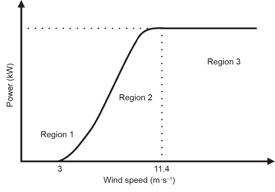
Fig. 1. The power curve of the NREL offshore 5 MW wind turbine.
According to the power curve, the wind turbine operating conditions are typically divided into three regions.
(1)Region 1: The wind speed is very low (< 3 m·s−1 for a 5 MW wind turbine). The turbine is stopped from rotating by a mechanical brake.
(2)Region 2: The wind speed is not strong, and the goal is to capture maximum power from the wind, that is, to obtain the maximum aerodynamic coefficient.
(3)Region 2 ½: This is a transition region between Region 2 and Region 3. The objective in this region is to reach the rated power when approaching the rated wind speed.
(4)Region 3: The wind speed is high. The objective is to achieve the rated power and rotor speed. The aerodynamic power captured by the rotor (Pwind) is given by the following equation [4]:

where R is the rotor radius; ρ is the air density, v is the wind speed; and the power coefficient Cp, which represents the percentage of power capture by the turbine, is a nonlinear function of the tipspeed ratio (TSR) λ and the pitch angle β. It is usually represented by a look-up table, which can be obtained from field test data. The TSR is calculated as follows:

where ω is the rotor speed.
Taking a 5 MW wind turbine as an example, the power coefficient curve is shown in Fig. 2. The figure shows that the maximum Cp is 0.4806 when the pitch angle is −1° and the TSR is close to 7. Since the primary objective in Region 2 is to capture the maximum energy from the wind, Fig. 2 indicates that the best choice is to maintain the pitch angle at the optimal value of −1°, and attempt to keep the TSR to the optimal value of 7. Eq. (2) shows that the TSR is indeed the ratio between rotor speed and wind speed. Maintaining a constant TSR means changing the rotor speed along with the fluctuating wind speed. The most-used method to track the optimal TSR is torque control, which is discussed in Section 3.2.
《Fig. 2》

Fig. 2. Power coefficient curve of a 5 MW wind turbine. (a) Cp surface; (b) Cp contour.
《2.3. Dynamic model》
2.3. Dynamic model
The aeroelastics of wind turbines are highly nonlinear, so we use the FAST code developed by NREL [11] to develop the numerical model of the wind turbine.
The nonlinear aeroelastic equation of motion for the wind turbine has the following form [11]:

where M is the mass matrix, f is the nonlinear forcing function vector that contains the stiffness and damping effects, q is the response vector, u is the vector of control inputs, ud is the vector of wind input disturbance, and t is time. The variable f is determined by AeroDyn, in which the underlying physics is based on BEM theory. Eq. (3) is then linearized by FAST code in the operating condition according to small perturbation theory. A linearized equation of motion can be obtained as follows:

 are, respectively, the linearized mass, damping, and stiffness matrices;
  is the control input vector; and
  is the wind disturbance vector.
A simple reduced-order linearized model can be obtained from a nonlinear turbine if certain degrees of freedom (DOFs) are switched on. A wind turbine system is a periodically rotating system even when the system is at the steady state because of the wind shear and tower shadow effects. Thus, the first step of the linearization is to obtain a series of linearized state-space models at a number of equally spaced rotor azimuths in one revolution. All the states are defined in the rotating coordinates. The state-space form representations are then averaged from all the linearization sets obtained. Finally, a linear time-invariant (LTI) state-space form representation can be obtained as follows:

where x = [qT, q. T]T is the state vector; A, B, C, and D are the state matrix, control input matrix, output matrix, and control input transmission matrix, respectively; Bd and Dd are the wind disturbance input matrix and the wind disturbance input transmission matrix, respectively; and y is the vector of output.
Multi-blade coordinate transformation
As mentioned earlier, a wind turbine is a periodic system due to wind shear and tower shadow effects. The dynamics of wind turbine rotor blades are generally expressed in rotating frames attached to the individual blades. However, the responses of rotor dynamics relative to the nacelle and tower must actually be considered as an integral response as a whole instead of as the individual response of each blade. Multi-blade coordinate transformation (MBC) can transform the dynamics of the rotating frame to those of the nonrotating frame (consistent with the fixed tower frame) and coherently interconnect the spinning rotor with the nacelle and tower. MBC was derived and first used in helicopter systems to analyze the flap motion-related stability [16].
The aforementioned LTI model is simple and is often adopted in collective pitch control strategy. Recent studies have found that MBC can reduce the variations between the different linearization results obtained at different azimuths, and therefore yields a better representation of the turbine dynamics [17]. MBC is widely used in individual pitch control strategy to better deal with periodic dynamics. A detailed transformation from rotational coordinates to fixed coordinates can be found in Ref. [18].
《2.4. Actuators》
2.4. Actuators
Three types of actuators are employed in wind turbine systems.The first type is the pitch actuator, which in the past was mostly hydraulic. At present, electromechanical pitch actuators have been adopted in many utility-scale land-based wind turbines. A change in blade pitch angle can produce an aerodynamic attack angle change and can therefore change the aerodynamic torque and force. Commercial turbines nowadays are equipped with individual pitch actuators for the independent adjustment of each blade, which yields the major advantage of eliminating asymmetric blade loads. In general, there is a delay between the pitch command and the actual pitch, which is usually chosen as a first-order transfer function. The second type of actuator is the generator actuator, which can be set to track a reference torque or load. The generator actuator uses the generator and power electronics to decide how much torque to extract from the turbine by the separation of magnets in the generator stator and rotor [6]. The net torque on the rotor is the difference between the torque induced by wind in the low-speed shaft and the load torque induced by the generator in the high-speed shaft. Therefore, the generator torque influences the acceleration of the rotor. The third type of actuator is the yaw actuator, which is generally motor-based. It is mounted such that it can navigate the whole nacelle to face to the wind direction. The yaw rate cannot be high due to gyroscopic forces. The yaw rate is typically less than 1°·s−1.
《3.Wind turbine control approaches and applications》
3.Wind turbine control approaches and applications
Wind turbines have different control objectives in different operating regions. The general strategy is to maximize energy in Region 2 and limit the power or rotor speed in Region 3.
《3.1. Pitch control》
3.1. Pitch control
Pitch control is often adopted in Region 3 to regulate power or to mitigate structural loads. It is the most widely studied subject in wind turbine control. There are two forms of pitch control: collective pitch and individual pitch. Collective pitch means that the pitch angles of all two or three blades change at the same angle each time. Individual pitch means that the pitch angles of all two or three blades change at different angles based on individual needs, which mostly depend on the blade azimuth when the rotor is rotating. The function of collective pitch is often to regulate power and rotor speed and to mitigate symmetric blade loads, while the direct goal of individual pitch is to mitigate asymmetric blade loads.
The intuitive idea for collective pitch control is to adopt a singleinput single-output (SISO) feedback loop to track the reference in Region 3 when the wind speed is time-varying. The reference signal can be the rated rotor speed or the rated power. The most commonly used approach in industry is to track the rated rotor speed using a proportional-integral-derivative (PID) controller. The rotor speed error between the nominal value and the rated value is fed back to the pitch actuator. The plant model is linearized from nonlinear dynamics when the system is at a one-equilibrium position, which means that there is no acceleration or deceleration of the rotor. The proportional, integral, and differential gains are tuned at one operating point. Nevertheless, owing to the time-varying nature of a wind turbine, the actual operating point keeps changing. The original proportional, integral, and differential gains cannot maintain the desired performance. Therefore, a gain-scheduling corrector is added to change the gains using the changing operating point [4].
The form of the gain scheduled proportional integral control can be written as follows:

where Δθ is the small perturbation of the blade pitch angle around the operating point, Δω is the error between the measured rotor speed and the rated set point value, and KP and KI are the proportional and integral gains tuned at the operating points. The function of the gain correction factor GS(θ) is to change the gains when the wind speed is time varying. The expression of GS(θ) is shown as follows [4]:

where θ is the blade pitch angle and θk is the blade pitch angle at which the pitch sensitivity value is doubled from its value at the rated operating point. The gain-scheduling part is derived from the pitch sensitivity, which is expressed as the sensitivity of the aerodynamic power to the rotor collective blade pitch.
It is worth noting that, strictly speaking, the relation between the pitch sensitivity and the pitch angle is nonlinear. Thus, disturbance effects may not be perfectly cancelled out. In a recent study, the low frequencies content in wind excitation was rejected with the combination of gain-scheduling PID and disturbance observer-based control [19]. The results showed that the power and speed regulation could be further enhanced. In addition to PID-type control approaches, speed regulation can be achieved from adaptive control, in which the model parameters of the wind turbine can be unknown [20]. The reference signal is simply the rated generator speed. The output of the nominal plant is forced to track the reference in the presence of various internal and external uncertainties. All of the aforementioned methods use the generator speed error as the measurement and feedback to obtain the blade pitch angle.
Wind turbine control loops are actually multi-input multi-output (MIMO) systems. Traditional PID control may not deal with such a system effectively. In particular, when the control objective encompasses mitigating loads on individual blades, a multivariate system must be decoupled into two SISO systems to facilitate the usage of PID control. However, the system may not be perfectly decoupled, especially at high frequencies. The usage of the SISO control method inevitably sacrifices some performance. In essence, many aspects in wind turbine control need to be dealt with at the same time, and some even conflict with each other, such as power capture, load mitigation, and pitch activity. The collective speed control loop is coupled with the tower loads because the regulation of the generator speed may excite the first fore-aft and side-side tower modes. In addition, the mitigation of blade loads requires more activity of the pitch actuator, although the actuator has its own mechanical limitation as well. Otherwise, the reduction of loads will also influence the power capture. Therefore, a strategy that can deal with multiple objectives is desirable.
The most common methods for MIMO systems are disturbance accommodating control (DAC)/linear quadratic regulator (LQR)/linear quadratic Gaussian (LQG), model predictive control (MPC), and the H2/H∞ method.
3.1.1. Disturbance accommodating control
To deal with speed regulation and load mitigation at the same time, DAC is a widely employed method that is implemented in conjunction with the LQR method. A trade-off between different objectives can be made through the proper selection of weighting functions. Johnson [21–24] first introduced the concept of DAC, and Balas et al. [25,26] later utilized this concept for a wind turbine field. In DAC, the wind disturbance is assumed to be the difference in wind speed between the nominal condition and the operating condition. The disturbance model can thus be augmented with the plant model to estimate the disturbance and state variables. The full state feedback control gain can be computed by the LQR method [27].The DAC block diagram is shown in Fig. 3.
《Fig. 3》

Fig. 3. Disturbance accommodating control block diagram. G is the state gain, Gd is the disturbance state gain, is the state estimation, and is the disturbance state estimation.
The very first step of DAC is deciding the model of disturbance.The disturbance model can be expressed in the state-space form:

Where zd is the disturbance state, and F and Θ are state matrices. A state estimator can estimate the state variables and disturbance that cannot be measured, such as

where  and
and  are the estimates of x, ud, zd, and y, respectively; and K1 and K2 can be determined by pole placement theory, ensuring that the system characteristics of the estimator are satisfied. The DAC control law is given as follows:

where G is the state gain and Gd is the disturbance state gain. The state gain can be obtained by the LQR method, and the disturbance state gain can be obtained by minimizing the L2 norm ||BGd + BdΘ||. Here, in practice, x and zd are the estimated values.
In practice, collective pitch control and individual pitch control require different choices of models of incoming wind, which means that F and Θ are different. Since the collective pitch can only adjust the uniform and symmetric component, in this scenario, the disturbance is modeled as a uniform step signal, which can be seen as wind rising from one magnitude to another at every sampling interval. F and Θ are assumed to be known as
F = 0, Θ = 1 (11)
In contrast, the individual pitch can adjust the asymmetric component. Due to the vertical wind shear variation across the rotor plane, the turbine blades experience periodic sinusoidal components [7]. The choice of F and Θ can be

where ωIP is the once-per-revolution (1P) rotor speed in rad·s−1. Although higher frequencies can also be involved in matrix F, here we just take the 1P frequency as the example. In this way, the 1P frequency of the load can be mitigated.
Further explorations of DAC have been made in recent years. Since the periodic dynamics in a wind turbine arise from both structural and aerodynamic effects, Stol and Balas [28] studied periodic DAC, which uses the time-varying feedback gain within a fixed time period. The results showed that the blade load attenuation level was improved compared with the PID and time-invariant DAC controller without a sacrifice of speed regulation. The transient response of the blade load that was introduced by the Rankine vortex in the flow was mitigated by considering the coherent turbulent inflow conception in DAC in order to improve the wind disturbance rejection effects [29,30]. In theory, the collective pitch controller can only reduce the blade symmetric loads because only horizontal uniform disturbances can be taken care of in this case. In the individual pitch control for mitigating the blade asymmetric loads, the wind disturbances were modeled as the combination of a collective horizontal component and an asymmetric linear shear component [31,32]. The harmonic component in the local blade wind speed can be included in the disturbance model, which thus yields periodic disturbance rejection. The results showed 1P and 2P load reduction and better rotor speed regulation. To compute the generalized inverse in order to minimize the disturbance, three methods were investigated: the Moore-Penrose pseudoinverse, the Kronecker product, and the D-1 method [33]. Pace et al. [34] expanded DAC to prevent emergency shutdowns by wind turbine overspeeds by using light imaging, detection, and ranging (LIDAR) to detect extreme events. The key idea was to switch the operational controller from the baseline controller (a gain-scheduled DAC) to an extreme event controller (areduced generator speed-tracking DAC). The results showed that the switching controller improved the mean power. In addition, for offshore wind turbines, the wave disturbance can be included in DAC, in which the platform yaw DOF can be modeled in the disturbance model. The results showed improved power and speed regulation [5].
3.1.2. Model predictive control
MPC is an advanced control method that can make use of the predictive model and current measurements to obtain the control signal by minimizing a cost function. MPC can use the model to predict the process output in the future horizon, and can calculate a control sequence by minimizing the desired cost function with constraints existing in the inputs and outputs. This is a receding strategy in that at each step, a few future control signals are calculated, but only the first calculated control sequence is applied to the real plant [35]. A number of MPC approaches tailored for wind turbines have been presented in recent years.
MPC can be mathematically divided into unconstrained and constrained approaches. Without loss of generality, the constrained optimization problem is illustrated here to calculate the optimal control inputs  in order to minimize the cost function J(zK ), which is characterized based on the system-level requirements. The cost function J(zk) is defined as the sum of all derivations of the system output y from the reference value r over the entire prediction horizon p weighted with Q, and the sum of all changes in the control input u over the entire control horizon m weighed with R. ·(k + i | k) denotes the predicted value of (·) at the ith prediction horizon step based on the information at time k. In general, the state and disturbance information at time k can be extracted using the state estimator. MPC solves the quadratic equations as follows:
Find to minimize

where k is the current control interval, p is the prediction horizon, m is the control horizon, and

All the MPC algorithms for wind turbines possess common elements, whereas different options can be chosen for each element, giving rise to different algorithms. These elements are: ① the prediction model, ② the objective function, and ③ the control law [35].
The prediction model is the cornerstone of MPC. A good design needs an accurate representation of the necessary mechanisms that can fully capture the process dynamics and allow the predictions to be calculated. In the literature, both linear MPC and nonlinear MPC are derived to solve the same optimal problem in terms of the basic concept, whereas the models and optimization algorithms are different. A linear model derived from simple physics including the aerodynamics, drive train, and generator was introduced in Ref. [36]. This model was effective in mitigating drive train loads and maximizing energy capture. Later, another linear model that also included the tower DOF showed good regulation of rotor speed, tower loads, and drive-train torsional loads in all operating regions [37]. Schlipf et al. [38] used FAST code to directly linearize the model from nonlinear dynamics. This provided another effective way to obtain the linear model, which can easily include more DOFs. All of the aforementioned linear MPC approaches used one model for all the operating points. A scheduled MPC, including multiple linear models in different operating points, was used for rotor speed regulation and drivetrain load mitigation [39]. All of the linear models produced the output at the same time, and the final output was computed by the weighted sum method, where the weightings were chosen based on the estimated wind speed.
MPC based on the nonlinear model is certainly promising because of the direct inclusion of inherent aerodynamic nonlinearities [38,40,41]. One way to obtain the nonlinear model is from aeroelastic simulators, such as FAST code, which use BEM to calculate the effect of the wind field on the turbine. Although the response predictions are accurate, the computation has to be carried out iteratively and thus becomes more costly. A slightly different way of incorporating nonlinear dynamics is reduced-order modeling by deriving the nonlinear aerodynamic thrust and torque using a look-up table [40]. An explicit comparison between the linear model predictive control (LMPC) and nonlinear model predictive control (NMPC) is presented in Ref. [38]. The LMPC used a linearized model of one operating point while the NMPC was linearized for each prediction step. The results showed that the NMPC achieved better performance even when the wind speed was far from the operating point.
Another important part of the prediction is how to represent the state variables and the disturbance. In the past, wind speed was generally assumed to be an unmeasured variable and was calculated with the Kalman filter (for linear systems) or the extended Kalman filter (for nonlinear systems) [36,39]. With the recent development of the wind speed sensor LIDAR, the state prediction in an MPC problem can be simplified and can become more accurate. LIDAR is mounted on the nacelle and can measure upcoming wind speed [42]. The investigation showed that the performance of a linear MPC could be enhanced quite significantly, if a perfect wind speed preview was obtained [42,43]. Another study showed that a nonlinear MPC could enhance the load conditions on the tower and blades, and led to the reduction of the pitch activity with the preview LIDAR measurements [40]. Although some studies indicated that the wind speed preview by LIDAR was not perfectly accurate [44], it was demonstrated that even with imperfect but realistic LIDAR measurements, load mitigation and pitch activity reduction could be realized with nonlinear MPC [45]. In such a situation, a time-varying model predictive controller was proposed to be used with preview measurements of the wind speed approaching the rotor. Two kinds of measurements were compared: the undistorted measurements at the position rotating with blades, and the measurements that were acquired at the same position but that included distortion characteristics. Both were incorporated into MPC and compared with a previous study using an H∞ preview controller. The results showed surprisingly better performance with MPC, even with distorted LIDAR measurements, compared with the H∞ preview controller. Thus, the performance can be enhanced when the future variable can be accurately predicted [42].
MPC has additional advantages over some other methods when applied to a wind turbine by employing the objective function and constraints. MPC can easily deal with the multivariable problem when several conflicting performance indices exist, such as balancing loads on the tower and blades [40]. Moreover, the constraints in the control input introduced by the pitch actuator can be easily considered in the control law design stage [40]. The fatigue damage dynamics can be integrated into the control design to account for the fatigue mechanism of the material in the objective function [46]. In addition, the robustness of the controller can be improved by including the dynamics inflow in the MPC prediction model [47]. In most of the literature [36,40,42,48], the optimization problem in MPC was solved by the weighted sum method, which combines several different cost functions into one cost function. The study in Ref. [49] investigated the tuning strategy based on the computation of sensitivity tables, aiming to achieve a trade-off between different weights in the multi-objective cost function so that the performance could be optimized with respect to five defined measures: power variation, pitch usage, tower displacement, drivetrain twist, and the frequency of violating the nominal power limit. In the weight tuning process, multi-objective MPC with Pareto curves is subsequently introduced to attain a better balance of different conflicting objectives, such as power capture and tower fore-aft fatigue load in the entire operating region [50].
3.1.3. Robust H2/H∞ control
For a typical three-blade wind turbine, an effective way to reject the periodic load disturbances is to mitigate loads at the nP frequencies (where P is the per revolution frequency and n = 1, 2, 3, ...). The periodic disturbances on the loads come from wind shear, the tower shadow, and the centrifugal force. It is typical to only consider the periodic effects at low frequencies, that is, 1P, 2P, 3P, and 4P. Further reduction of loads at higher frequencies requires higher pitch rates, which actually increase the loading in the pitch actuator and therefore reduce its lifespan. In H2/H∞ methods, using the weighting function to perform loop shaping is a promising way to deal with the performance within a certain bandwidth. Control efforts and system performances can be penalized directly by this mixed-sensitivity optimization problem.
A typical example using H∞ control is shown in Fig. 4. There are two control loops in the turbine pitch system: One is the collective pitch loop regulating the generator speed, which provides the collective signal; the other is the individual pitch loop, which provides a small modification summed with the collective pitch based on the blade azimuth angle in the rotor plane. In the individual control loop, the blade root moments at each blade root are transformed to tilt and yaw moments in the non-rotating coordinate by MBC transformation. The individual pitch controller can be a multivariate H∞ controller. The tilt and yaw pitch angles are transformed back to the rotating coordinate by the inverse MBC transformation, and are then summed with the collective pitch signal.
《Fig. 4》
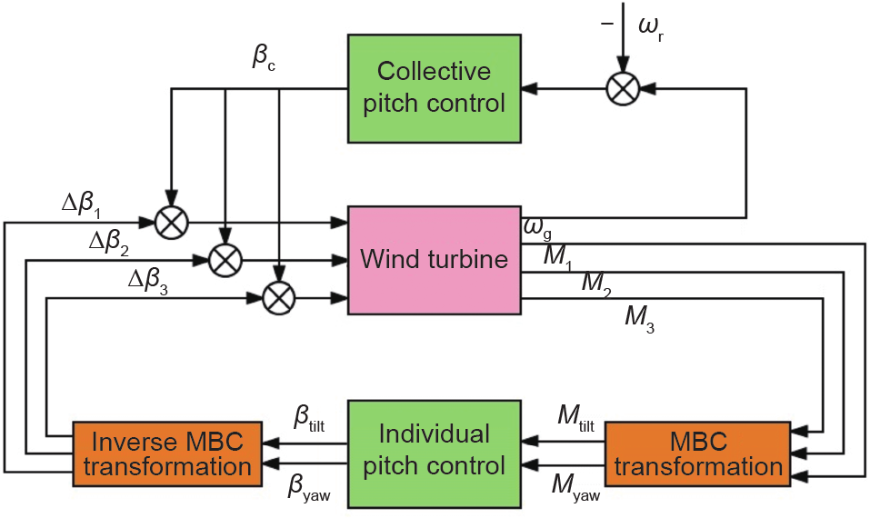
Fig. 4. An augmented control block diagram of collective and individual control. βc is the collective pitch angle; ωr is the rated generator speed; ωg is the output generator speed; M1 , M2 , and M3 are the root moments at blade1, 2, and 3; Mtitle and Myaw are title and yaw moments after MBC transformation.
The general H∞ control configuration is shown in Fig. 5, where P is the generalized plant model, which includes the plant, disturbance model, and interconnection structure between the plant and controller. The interconnection structure can include the weighting functions to facilitate further loop shaping. The variable w is the exogenous input, which corresponds to the periodic disturbances; z is the exogenous output, which refers to the tracking error to be minimized between the nominal generator speed and the rated generator speed; vi is the controller input for the general configuration, such as commands, measured plant outputs, and so forth; and u is the control input. The optimal H∞ control yields a feedback controller K to minimize the tracking error, and mitigates the effects of wind disturbances to the blade flap loads on the 1P, 2P, 3P, and 4P frequencies.
《Fig. 5》

Fig. 5. The H∞ control block configuration. K is the feedback controller.
The optimization process minimizes the infinity norm of the weighted closed-loop transfer function S (i.e., the output sensitivity function), KS, and T (i.e., the complementary input sensitivity function) as follows:

where

The sensitivity function S is a very good indicator of the closedloop performance, for both SISO and MIMO systems. The main advantage of considering S is that, since ideally we want S to be small, it is sufficient to consider just its magnitude | S |, without considering its phase.
The weighting function can be properly chosen to make a tradeoff between multivariate conflicting performance indices; this is called the mixed-sensitivity optimization problem. For example, to achieve robustness or to avoid too-large input signals, it may be desirable to place bounds on the transfer function KS. Furthermore, an upper bound may be specified on the magnitude of T to ensure that L rolls off sufficiently rapidly at high frequencies. In the sensitivity function, a high gain means a large disturbance rejection. It is worth noting that after MBC transformation, the original 1P, 2P, 3P, … frequencies in the rotating frame are changed to 0P, 3P, 6P, … frequencies. Therefore, it is necessary to concentrate on the reduction of low frequencies and 3P frequency performances. For the selection of the weighting function W1, low frequencies (0P) have the high gain and 3P frequency has an inverted notch. High frequency is not commonly considered because of the limitation of the pitch actuator. The weighting function W2 is selected to guarantee that the actuator is functional in the proper bandwidth. So W2 is always a high pass filter, which has a low gain below the actuator bandwidth and a high gain beyond the actuator bandwidth. The cross frequency should be in the middle of the bandwidth. The weighting function W3 is chosen as the empty matrix, which means that there is no plenary on T.
A linear matrix inequalities (LMI) formulation of the control problem is able to optimize a linear parameter-varying controller by minimizing the H2/H∞ norm. The controller in Ref. [51] considered the blades, shaft, and tower DOFs and showed enhanced performance compared with gain-scheduling LQG and a proportionalintegral (PI) controller. Later, a robust LMI-based controller was designed to facilitate the additional constraints under the entire operating conditions. This controller can include the parametric uncertainties in the model with the presence of structural uncertainties [52]. In Ref. [53], it was shown that generator speed control could increase the closed-loop disturbance rejection bandwidth and the tower fore-aft displacement. Both performances can be enhanced with the collective H∞ multi-input single-output controller. By considering that significant coupling exists between the yaw and tilt modes after MBC transformation in the individual pitch loops, and that the modes of the blade vary with the rotational frequency, a frequency-related MIMO plant was constructed to facilitate the H∞ mixed-sensitivity optimization problem [54]. The periodic disturbance model was included in the control design stage, but the results showed that it only had an obvious contribution in steady winds. Even at low-turbulence wind disturbances, it did not lead to the expected load mitigation. This was because the turbulence had wide spectrum energy and the reductions at the multiple frequencies were not important [55].
3.1.4. Combined feedforward/feedback control
The control approaches reviewed in the preceding sub-sections are based on feedback. However, there are several issues in wind turbine control that call for the involvement of feedforward. For example, there may be a time delay between sensing a wind gust and the subsequent mechanical adjustment of the rotor torque response, which can affect the effectiveness of the controller. Recently, researchers have been studying feedforward strategy, which is able to “foresee” the incoming wind speed, and which facilitates the input behavior before future wind hits the turbine. The LIDAR system can provide wind field measurements ahead of the rotor plane. The preview of the wind sequence can be fed to the loop, enabling the controller to take precautions before the corresponding wind event arrives. Furthermore, feedforward control can be combined with feedback control in order to handle multivariate objectives simultaneously [56,57]. The structure of combined feedforward/feedback control is shown in Fig. 6.
《Fig. 6》

Fig. 6. Combined feedforward/feedback control architecture.
An initial study of feedforward control used wind speed estimation based on the reconstruction of aerodynamic torque from measurements and on a prior knowledge of rotor behavior [58]. The goal was to reject wind disturbances and simultaneously regulate rotor speed when wind turbulences and wind gusts were present. The results showed that the feedforward method was promising to reduce speed variation by 30%–40%. Later, a combined feedforward and feedback control was developed to include other goals, such as load reduction [59]. The feedback part was an optimal LQG controller that minimized the yaw and tilt modes through individual pitch control by enhancing the reduction of the 1P and 3P loads. The feedforward part was proposed to reject the influence of the low-frequency component of the wind on the rotor moments. Here, wind speed was estimated by the Kalman filter, in which the random walks wind model was augmented with the turbine states. The predictions of future wind were not needed. In contrast to the LQG feedback loop, the H∞ control method, which tries to minimize the preview local wind speed to the individual blade root bending moment, is more straightforward because it considers the constraints in the pitch actuator. In Ref. [60], preview control was applied to two models: the non-MBC model and the MBC model. The results showed that significant improvement in load mitigation can be realized, and that the reduction level was influenced by the accuracy of the wind preview and the available pitch rate. In Ref. [61], this concept was explored further; a non-causal series expansion was used as the pitch feedforward controller with the measurement of incoming wind speed. The results showed that reduced blade flap and tower base fore-aft damage equivalent load could be achieved, while the pitch rate was significantly increased. In another study [62], it was shown that an adaptive strategy, the filtered-x recursive least squares (FX-RLS)based feedforward method with LIDAR, could improve disturbance rejection and vibration suppression. The controller was able to improve tower and blade bending moments, rotor speed regulation, and pitch actuator usage, with a small sacrifice of power capture. Although feedforward control can benefit from LIDAR measurements to achieve multivariable objectives simultaneously, the LIDAR wind speed measurement error caused by LIDAR distortion and wind evolution can severely influence its performance. One possible solution involves adding an optimal filter after wind measurements, which can reduce the error [63]. The effectiveness of feedforward control with LIDAR has been validated by a filed test conducted by NREL [64,65]. The experiment showed enhancement of rotor speed regulation and load reduction, which can extend turbine life and reduce energy cost.
《3.2. Torque control》
3.2. Torque control
When the wind level is in Region 2, torque control is the main control strategy. The most challenging aspect of wind turbine torque control involves the uncertainties in aerodynamics. According to Ref. [7], the generator torque (τ) that leads to the optimal TSR is expressed as follows:

where ωg is the generator speed and kg is an optimal constant:

and where R is the rotor radius, ρ is the air density, Cpmax is the maximum power coefficient of the turbine, and λ* is the optimal TSR that leads to Cpmax .
Johnson [66] utilized adaptive control to reduce the negative effects of uncertainties. An adaption law was designed to optimize the gain for the maximum energy capture under time-varying turbulent wind fields. The effectiveness of the adaptive controller was tested in real field tests [66]. The stability analysis was further investigated in Ref. [67]. From the Cp surface, it is clear that the maximum aerodynamic coefficient is obtained when the optimal TSR is obtained. The adaptive control in Ref. [68] tracked the optimal TSR under the time-varying wind conditions with wind speed estimated by the state estimator. Another study on optimizing power capture by tracking the optimal aerodynamic torque is illustrated in Ref. [69], in which a second-order sliding model observer is used to deal with model uncertainties and electric grid disturbances. Nonlinear robust control can provide a balance for conversion efficiency and torque oscillation smoothing. De Corcuera et al. [53] discussed how two SISO H∞ torque controllers can be used to reduce the wind effect on the drive-train mode and tower side-side mode, respectively. In addition to these SISO-type torque controllers, a multivariable strategy was developed by combining nonlinear dynamics state feedback control for torque control with a linear strategy for pitch control [70]. The results showed that this strategy could lead to a trade-off between power regulation and rotor speed regulation.
《3.3. Yaw control》
3.3. Yaw control
Active yaw control can direct the turbine rotor to face into the wind direction. The sensor mounted in the nacelle can measure the wind direction and determine the control signal of the yaw controller. The yaw motor is triggered when the yaw error exceeds a certain amount, and it will yaw at a constant rate in the ideal direction to capture the maximum power. Yaw control can help to reduce the structural loads. For example, with a periodic linear quadratic controller used as a suspension system, the lateral tower motion, which is closely related to the yaw dynamics, can be reduced [71]. An optimal yaw control that takes wake effects into account is presented in Ref. [72]; here, the controller used an internal parametric model for wake effects to predict turbine electrical energy production levels as a function of yaw angles. When simulated using computational fluid dynamics, the results indicated increased energy production and an additional load reduction. A very recent study of yaw control for wind farms is presented in Refs. [73,74]. Yaw control can deflect the wake in the near-wake region and change the wake trajectory downwind. Hence, it is possible to use yaw control in individual turbines to manage the wind farm wake behavior and to improve the overall performance at the wind farm level. A further study about wind plant annual energy production (AEP) using yaw-based wake steering control and layout changes is presented in Ref. [75]; the outcome showed a 5% AEP enhancement.
《3.4. Passive control methods》
3.4. Passive control methods
Reducing the loads of various components of wind turbines enhances reliability and durability. Passive controls can be adopted to facilitate such a goal. In Ref. [76], a TMD was placed at the top of the tower to reduce the tower top vibration. In Ref. [77], two independent single-DOF TMDs were placed in the nacelle to separately deal with the fore-aft direction motion and the side-side direction motion.
With the increasing size of wind turbine blades, blade load mitigation becomes more and more important. The so-called smart rotor concept is built on a blade that is equipped with several control devices that can locally change the lift profile of the blade. This technology is inspired by applications in aircraft and rotorcraft systems. Trailing edge flaps and strain sensors can be used to facilitate feedback control. The experiments in Ref. [78] demonstrated a proof-ofconcept study of the smart rotor, which effectively reduced 1P and 3P frequencies.
The microtab is another device that controls the aerodynamics in order to achieve load mitigation on the blades [79]. Microtabs are small translational devices that are attached near the trailing edge of an airfoil. They are deployed approximately normal to the surface, and have a maximum deployment height on the order of the rotor blades. These structures influence the lift with the change of trailing edge flow development and thus affect the effective camber of the airfoil. A prototype can be found in Ref. [79], which presents a dynamic model representing the influence of microtabs on the aerodynamics of a local airfoil. The frequency response of the blade loads was investigated in order to guide its design to reject loads in various frequency regions. Such a device could extend the lifespan of blades [80]. This research was extended in Ref. [81], in which a non-traditional microtab was analyzed in terms of the discontinuous, draft, and lower and upper surface tab deployment effects on the airfoil.
《3.5. Recent developments and future directions》
3.5. Recent developments and future directions
At present, many researchers are working on various aspects of wind turbine control, as reviewed above. In addition, there is a new trend of improving performance from a global wind farm perspective. Individual turbine behavior can be coordinated with the performance of the whole wind farm since neighboring turbines influence each other owing to wake effects. For example, recent work has provided a proof of concept for a data-driven optimization control scheme that employs yaw control to change the wake trajectory in a high-fidelity wind plant simulation [65,72,74,75]. Future work may concentrate on the more accurate analysis of wake effects, such as the delays produced by the propagation of the wake through the wind field. Control design with LIDAR is another promising future direction that provides measurements of the flow and an estimation of the wake locations for use in control loops. Recent work in this area has verified its effectiveness in load mitigation and power capture [38,40,42,44,45,57,62,64,65]. The use of LIDAR is being field-tested [82].
《4.Summary》
4.Summary
This article provided a review of the control methods that have been developed for the optimization of power capture and load reduction in wind turbine components under time-varying turbulent wind fields. The dynamics and modeling of wind turbine systems, which encompass the mathematical representation of systems, power curves, operating conditions, MBC transformation, and actuators for collective or individual control, were summarized first. Three separate control loops—pitch control, torque control, and yaw control—were discussed, with the main focus being on pitch control strategies. Passive control approaches and ongoing developments were briefly reviewed as well.
《Acknowledgment》
Acknowledgment
This work is supported in part by the US National Science Foundation (CMMI1300236).
《Compliance with ethics guidelines》
Compliance with ethics guidelines
Yuan Yuan and Jiong Tang declare that they have no conflict of interest or financial conflicts to disclose.


 京公网安备 11010502051620号


