《1.   Introduction》

1.   Introduction

The life cycle of a life-line structure such as a long-span bridge is an integrative process in which each stage of the bridge’s existence should be thoroughly checked, from its construction to the designed life-period. In the construction stage, the structural system of a bridge differs from in the in-service design, leading to additional design checks that are performed under critical erection conditions [1]. In the case of long-span flexible bridges, these checks are commonly conducted against critical wind conditions. This ensures safety and serviceability throughout the construction and in-service periods by limiting the response by which residual forces are stored in the structure. Fluid-structure interaction (FSI) due to gusty wind is a complex phenomenon, and is described by several approaches and models. In the case of bridge decks, the   FSI is commonly simulated by wind-tunnel experiments or semianalytical models based on the theory of aeroelasticity, supplemented by wind-tunnel deliverables [2–6]. Within the last two decades, numerical approaches based on computational fluid dynamics (CFD) [7–9] have also received considerable attention. With different sets of assumptions, semi-analytical models are based on the analytical solutions from flat-plate aerodynamics. With the introduction of modification coefficients based on experiments, they model the complex unsteady behavior of bluff bodies. The two main assumptions under which semi-analytical aerodynamic models are developed are the  quasi-steady  assumption  and the linear unsteady assumption. Within the quasi-steady assumption for bridge aerodynamics, fluid memory is neglected and aerodynamic nonlinearity is taken into account. Utilizing the linear unsteady assumption, the aerodynamic forces can be separated into static, buffeting, and self-excited force components in order to unveil the complex behavior of bluff body aerodynamics  in a linear fashion. In the latter assumption, the buffeting and the self-excited forces are considered to be dependent on the frequency of the wind fluctuations and on structural motion (i.e., fluid memory), respectively. Fluid memory is taken into account through frequency-dependent coefficients such as aerodynamic admittance functions and flutter derivatives.

Eight semi-analytical models in the time domain are considered within this study, including the quasi-steady (QS), linear quasisteady (LQS), linear unsteady (LU), corrected quasi-steady (CQS), modified quasi-steady (MQS), mode-by-mode (MBM), complex mode-by-mode (CMBM), and hybrid nonlinear (HNL) models. The QS model considers the aerodynamic nonlinearity while neglecting the fluid memory in the self-excited and buffeting forces. The simplest model may be the LQS model, which is linear and which does not consider the unsteadiness of the aerodynamic forces [10,11]. The LU model takes the linear fluid memory into account; that is,  it is based on the linear unsteady assumption [2–4]. Since the aerodynamic forces are of a mixed nature in the LU model, including timeand frequency-dependent terms, a rational approximation using transfer functions is required for the transformation in frequency-independent expressions. In bridge aerodynamics, it is common for the indicial [12,13] or impulse function formulation [14,15] to be employed as the approximation form of the transfer functions. The motivation of the CQS model [5] is to retain the advantage of the aerodynamic nonlinearity of the QS  model  and  to include the fluid memory in an averaged manner by introducing frequency-independent correction coefficients. The ambiguity in the torsional damping of the LQS model is accounted for in the MQS model by formulating the self-excited forces using frequency-independent coefficients based on the flutter derivatives [16]. In this way, the fluid memory is somewhat averaged. The time domain MBM model approximates the self-excited forces at the natural frequencies of oscillations, and ignores the aerodynamic coupling between modes. Aerodynamic coupling between modes is imperative in bridge aerodynamics since it is the main cause of coupled flutter instability. Using the complex modal decomposition method, the CMBM model [17] interpolates the flutter derivatives at the complex modal frequencies. The assumption in this model is that there are no significant peaks in the aerodynamic transfer function, except at the complex modal frequencies; however, aerodynamic coupling is preserved. Given the asymptotic property of the LU model to converge to the QS model for high reduced velocities, the HNL model [18,19] splits  the wind spectrum into lowand high-frequency components by     a cut-off frequency. For the low-frequency component, in which the quasi-steady assumption is valid, the QS model is used to model the aerodynamic forces; thus, the aerodynamic nonlinearity is considered. The effect of fluid memory in the aerodynamic forces for the high-frequency component is considerable; therefore, the LU model is employed. In this way, the advantages of the LU and QS models are exploited. Recently, several models have been developed   that  include   nonlinear  fluid   memory,   based  on   an approximation   of  the  aerodynamic  hysteretic  behavior   [20,21] and Volterra’s series [22]. However, these models will not be considered within this study, as the aerodynamic coefficients required for these models are not available for this case.

It is relevant here to review some of the comparative analyses that have been done in the field of semi-analytical aerodynamic modeling. Extensive analyses between the time and frequency domain for the QS and LU models are conducted in Refs. [23–25]. Various formulations, the computational efficiency, and algorithms for the indicial and impulse functions are compared in Refs. [15,26–28]. Wu and Kareem [29] performed a detailed analysis of the underlying assumptions for a flexible bridge deck section. They concluded that the fluid memory is one of the key factors in the aerodynamic response. However, they did not specify whether it was the fluid memory of the buffeting or that of the self-excited forces that influenced the total response. Nevertheless, an analysis without self-excited forces was performed from which the influence of the fluid memory of the buffeting forces on the response could be estimated without considering the effect of self-excited forces.

 The main goal of this study is to evaluate and quantify the effect of the assumptions of the studied semi-analytical models for the response of a cable-stayed bridge in the erection stage. The bridge was chosen to represent a typical bridge spanning a large river crossing. The deck is a concrete box girder, supported by post tensioned cables with a single cable plain. The typical construction methodology for these types of bridges is the balanced cantilevering method, in which the deck is erected in a segmental manner, symmetrical to the pylon. The maximum cantilever construction stage represents critical design conditions and should be accounted for accordingly. Compared with other studies dealing with closely related problematics, the  reference object is chosen to be rather stiff with a bluff cross-section. The research question is: Which model is sufficient to analyze this type of structure for design wind speeds?

Furthermore, a simplified method for the consideration of aerodynamic admittance is presented in Section 2.4.1. based on the convolution theorem. Since the wind fluctuations are generally available prior to the time integration,  rational  approximation  can be avoided by employing the method presented here. This method is tested and compared with the standard formulation using rational approximation in the LU model.

《2.   Semi-analytical aerodynamic models》

2.   Semi-analytical aerodynamic models

The wind-structure interaction is a complex three-dimensional (3D) phenomenon. However, most of the aerodynamic models are developed for two-dimensional (2D) sectional models, which are then applied to a 3D structure in order to simulate the full behavior. The governing equations of motion of a 3D linear structure discretized on finite elements using the mode generalized approach are given by the following:

where M, C, and K are the modal mass, damping, and stiffness matrices, respectively;    are the generalized displace ments as a function of time t along with their time derivatives, denoted with " . ”; and Ψ is  the  structural  mode  shape  matrix.  The generalized force vector  is  obtained from the nodal  force  fo  (the  subscript  o  is  used  for  the  full  order  system), where   is generally a nonlinear function of the aerodynamic loading, which includes static, buffeting (related to incoming wind fluctuations), and self-excited (related to bridge motion) components that are denoted as f_os, f_ob, and f_ose, respectively. Fig. 1 depicts a simplified three-degrees-of-freedom (3DOF) bridge  deck,  for  which  the  nodal  force  vector   includes the drag, lift, and moment components, respectively, and the   displacement vector   comprises the horizontal and vertical displacement and the rotation, respectively. The width of the bridge deck is denoted as B, and the wind acts with mean wind speed U with fluctuating components  u = u(t) and w = w(t) in the horizontal and vertical directions, respectively.

《Fig. 1》

Fig. 1. Coordinate system of wind fluctuations and aerodynamic forces acting on a bridge deck cross-section.

《2.1. Quasi-steady and linear quasi-steady models》

2.1. Quasi-steady and linear quasi-steady models

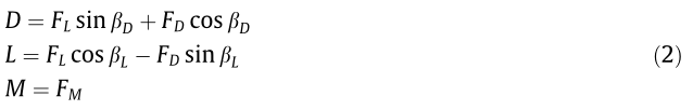
The QS model is based on the assumption that in each time step, the forces due to the FSI are the same as in an equivalent steady state at infinite time. Thus, the rise time of the aerodynamic forces is assumed to be instantaneous and the fluid memory effect is not considered. The main advantage of this model is its consideration of the aerodynamic nonlinearity: The wind coefficients depend on the instantaneous angle of attack, considering wind fluctuations and structural motion. The net forces acting on a bridge deck are defined in the subsequent form [6,10,11]:

Where

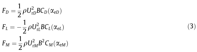
 In Eq. (3), q is the fluid density and are the static wind coefficients, which are nonlinear functions of the effective angle of attack,α_ej. The latter is obtained as follows:

where α_s is the static angle of attack, β_j is the dynamic angle of attack, and the resultant wind velocity, U_rj , is given by the following:

 for   The coefficient m_j defines the position of the aerodynamic center on the bridge deck, which will be discussed further in the following sections. The static wind coefficients from windtunnel experiments are usually given up to a certain angle of attack (±10°). Therefore, a linearized model with respect to the static angle of attack can be developed by employing Taylor’s approximation on Eq. (2) and using the hypothesis of small angles of attack—that is, by neglecting the quadratic velocity terms. Thus, the LQS model can be obtained as follows:

 Where  are  the static  wind coefficients  and  their derivatives    For  the  LQS  model,  the nodal force vector f_o can be obtained as a superposition of the buffeting and self-excited forces and a static force obtained from linear  or  nonlinear  aerostatic  analysis.  Implementation  of  the  LQS and QS models for discrete integration in the time domain is straightforward. It is further notable that neglecting the motionrelated terms in Eqs. (2) and (6) results in  what will be referred  to as the steady (ST) and linear steady (LST) models, respectively.

《2.2. Linear unsteady model》

2.2. Linear unsteady model

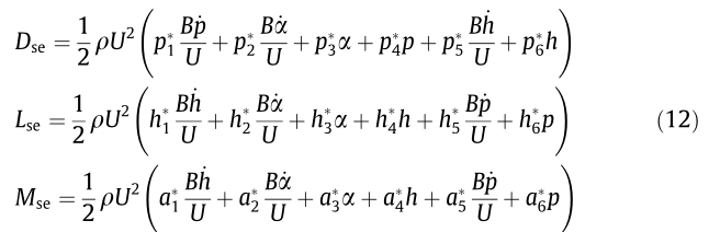
The models based on the quasi-steady theory do not take into account the unsteady behavior of the bluff body under laminar     or turbulent flow. In bridge aerodynamics, Davenport [4] and Scanlan [2,3] introduced an efficient way to treat unsteadies by including linear frequency-dependent coefficients. The self-excited forces are then described as a linear function of the motion and its frequency content, including the aerodynamic coupling between modes. The buffeting component of the force vector is modified   by introducing linear frequency-dependent coefficients between the wind fluctuations and the forces, which are commonly referred to as the aerodynamic admittance functions. The self-excited   forces in the extended Scanlan’s format are represented as follows [30,31]:

where are the flutter derivatives  dependent on  the reduced frequency K=Bω/U,  with  x being the circular frequency. The buffeting forces are given in the following subsequent form:

where are the aerodynamic admit-tance functions that are introduced to cover the unsteady effects of the  incoming wind  fluctuations. The  general  form  of  the aerodynamic admittance is complex; that is, where F and Gare the real and imaginary parts of the corresponding aerodynamic admittance function  respectively. This model neglects the aerodynamic nonlinearity; however, it takes the  linear  fluid  memory  into account. These relations are of a mixed nature since they contain frequencyand time-dependent terms; that is, and . In order to be able to solve the equation of motion in the time, these forces must be expressed in a pure time domain approximate formulation. In bridge aerodynamics, the impulse or indicial  (unit-step)  formulation  is  typically  employed.  Herein,  the approach based on impulse functions is adopted and the relations are given in Section S1.1 in Supplementary Information (SI).

《2.3. Corrected quasi-steady and modified quasi-steady models》

2.3. Corrected quasi-steady and modified quasi-steady models

Diana et al. [5] presented the CQS model in order to partially introduce unsteady effects into the QS model, while retaining the advantage  of  aerodynamic  nonlinearity.  Eq.  (3)  is  modified  as    represents a cor rected nonlinear static wind coefficient computed as follows:

where represents  the  frequency-dependent  correction  coefficients that are obtained from dynamic tests. Alternatively,  they can be computed from the aerodynamic derivatives for wind at a different angle of incidence as follows:

The flutter derivatives here are functions of the angle of attack and reduced frequency P_j = P_j(K, α), H_j = H_j(K, α), and A_j = A_j(K, α) for Since no  rational approximation  is employed, the  K^* coefficients are interpolated at the central reduced frequency K_c = 2πf_c/U, where f_c is the central frequency of the frequency content contributing to the response. In this case, f_c is computed as f_c =(f_h + f_α)/2, with f_h and f_α being the frequencies of the first vertical and  torsional  modes,  respectively.  Since  the  contribution  to the effective angle of attack of wind fluctuations and motion cannot   be separated, the correction coefficients account for the averaged fluid memory in the buffeting and self-excited forces. The implied assumption here is that the transfer functions of the self-excited and buffeting forces are essentially the same. There are studies   for bridge aerodynamics that have correlated the flutter derivatives and the admittance functions in an analytical and an experimental way (e.g., Refs. [32,33]). However, these correlations depend on the definition of the aerodynamic admittance based on the experimental method for its identification (complex [34] or spectral [35] method) and the analytical correlations do not hold for the flatplate analytical solution. Another ambiguous point in the QS models is the aerodynamic center, which is defined as m in Eq. (4). It is proposed in Ref. [5] and later restated in Ref. [19] that the aerodynamic center  can be  computed from  the flutter derivatives.  Comparing  terms  related  to  the  angular  velocity    in  Eqs.  (6)  and  (7) and substituting the derivatives of the  static  wind  coefficients  with their corresponding  terms  from  the  LU  model  (Eq. (7)) yield the aerodynamic center as follows:

For the aerodynamic center, it is noted in Ref. [19] that the flutter derivatives should be interpolated for reduced velocity: V _r = 2π/ K ≥ 15. However, this will be revisited in Section 3.4 for the flutter analysis.

The MQS model was developed in Ref. [16] in order to account for the ambiguity in the torsional damping in the LQS model that was introduced by the aerodynamic center. In the MQS model, the magnitude of the aerodynamic damping and stiffness are defined using the flutter derivatives, without considering the additional unsteady terms. The frequency-dependent self-excited forces in Eq. (7) can then be reduced in frequency-independent relations as follows:

where are frequency-independent coefficients; for they correspond to the aerodynamic damping, and for  ,  they  correspond  to  the  aerodynamic  stiffness.  The frequency-independent coefficients can be obtained either by using the linear least-square fit to the perimental data for the aerodynamic derivatives, or by using the secant approximation at the origin and an interpolated value for a chosen frequency of oscillation for an individual DOF. The relation of the frequency-independent coefficients with the rational coefficients of the approximate form of the impulse function formulation is  given in Section S1.2 in SI.   It is noted that the formulation of the MQS model given in Ref. [16] is in a slightly different form, as the frequency-independent coefficients  are  multiplied  or  divided  by  a  constant of  B or  U.  However,  this  is  an  arbitrary  choice  that  would only change  the  numerical  values  of  The  accuracy  of  the MQS model for predicting the response depends on the aerodynamic behavior of the cross-section, that is, on the goodness-of-fit of the flutter derivatives for the selected approximate form. If the flutter derivatives related to the aerodynamic damping have a somewhat linear trend and the flutter derivatives related to the aerodynamic stiffness have a quadratic trend, this model performs well for coefficients that are obtained using linear least-square fit. Otherwise, the secant approximation should be used for the reduced velocity range of interest.

For the buffeting forces, the LQS form is used in Ref. [16] without considering the aerodynamic admittance. Here, the fluid memory in the buffeting forces is considered using an alternative method described in the following section.

《2.4. Mode-by-mode and complex mode-by-mode models》

2.4. Mode-by-mode and complex mode-by-mode models

The MBM model ignores the aerodynamic coupling between modes. It is conventionally used for buffeting analysis in the frequency domain due to its simplicity, while the coupled flutter limit is determined using complex eigenvalue analysis. Transferring the system into modal coordinates for a bridge deck with length Ls, and moving the self-excited force vector on the left side of Eq. (1), yields the modal system stiffness matrix K_s = K_s(K) as K_s = K — K_ae, where K_ae = K_ae(K) represents the modal aerodynamic stiffness matrix. Similarly, the modal system damping matrix Cs = Cs(K) is obtained as Cs = C — Cae, where Cae = Cae(K) represents the modal aerodynamic damping matrix. Eq. (1) can then be expressed as follows:

The aerodynamic stiffness and damping matrices are given in Section S1.3 in SI. It is clear that the aerodynamic matrices are coupled and frequency-dependent. In the conventional frequencydomain formulation of the MBM model, the aerodynamic matrices are  decoupled   by   neglecting   the   off-diagonal   terms,   that   is, where I is the identity matrix and the superscript  “d” denotes the decoupled matrix. In order to solve the system in the time domain, the matrices need to be frequency-independent. Therefore, it is further assumed that there are no appreciable peaks in the transfer function of the system, except around the natural frequencies of the structure, and the matrices      are  assembled  by  interpolating  the  flutter derivatives at the reduced frequency corresponding to the natural frequencies of each mode. Alternatively, rational approximation with impulse functions can be used to cover the entire frequency range, without considering the coupling terms.

To account for the aerodynamic coupling and still solve a frequency-independent system for the self-excited forces, the CMBM model is introduced in Ref. [17] and revisited later on in Ref. [28]. The model is based on the complex decomposition technique of the state-space formulation of Eq. (13) as follows:

where vector y = y(t) contains the complex modal coordinates, is a matrix containing the complex eigenvalues, is a matrix containing the complex eigenvectors, and R is the input matrix. Since the preceding equation is decoupled and frequency-independent, it can be solved in the time domain if f_b is frequency-independent.   In the CMBM model, the frequency-dependent aerodynamic coefficients are interpolated at the complex eigenfrequencies. Compared with the LU model, this model can overestimate or underestimate the self-excited forces for frequencies of oscillation that are greater or smaller than the complex eigenfrequencies. The derivation of the CMBM model is given in Section S1.4 in SI.

2.4.1.    Method for the computation of unsteady buffeting forces

The force vector f_b in the CMBM model is still dependent on the reduced velocity, V_r, based on the wind frequency content. In Ref. [17], it is pointed out that the buffeting forces are computed in    the same way as in the LU model (presented in Section 2.2), that  is, with rational approximation, while in Ref. [28], the fluid memory is not included in the buffeting forces. Herein, a method will   be presented in order to avoid the rational approximation, which  is the motivation for the CMBM model.

The additional method utilizes the principles of the response of a stable linear system due to periodic inputs [36]. In this case, the buffeting force is the response, which is in fact stable, while the wind fluctuations are the input. Assuming that the vertical fluctuation w is a periodic signal, the lift-buffeting force L_bw = L_bw(t) can be obtained as follows:

where  “ · ”   denotes  point-wise  multiplication  and   F denotes  the   Fourier      transform.    The convolution  theorem  is  employed in  the  preceding equation, for  in  addition,  g = w and “ * ”  denotes the convolution  operation. In fact, the same theorem holds for the Laplace transform in the case of the solution of the convolution integral in the impulse function formulation (Eq. (S5) in SI). The difference in using the Fourier  transform  instead  of  the  Laplace  transform  for periodic input and stable output signals is that there is an additional assumption that the transient part (fluid memory) of the initial condition is zero. As shown later in Section 3.3, this influence is only a small initial part of the force time history. The wind fluctuations are commonly generated before solving Eqs. (1) or (14); therefore, the discrete Fourier transform (DFT) is employed for the discrete solution of the circular convolution implied in Eq. (15). The discrete lift force due to vertical gust L _bw [n] can be computed as follows:

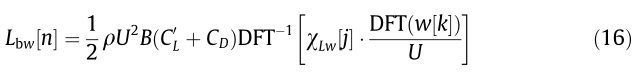
where  and N_s is the number of steps corresponding to the total time   being the integration time-step. The force and wind fluctuations are real signals and the force-wind relationship is a causal system. In order to ensure these two requirements, the admittance possesses Hermitian symmetry, and its imaginary part G is non-zero:

It is clear that instead of a rational approximation of vLw, interpolation or fitting in the frequency domain  can  be  used.  This is more convenient in bridge aerodynamics, especially for noisy   experimentally   obtained   admittance   functions   (e.g., Ref.[35]). This method could also be applied for admittance  func tions that are obtained from the spectral method with zero lag—that is, G = 0. However, it is noteworthy to mention that this situation implies that the admittance is a non-causal filter—that  is, the lift force depends on future  inputs.  Since  the  discrete  wind fluctuation signals are a superposition of the integer harmonic signals, the Gibbs effect and spectral leakage are avoided. Although this method for  computing  the  buffeting  forces  can also be applied in the  LU  or  HNL  models,  it  is  used  here  for the MQS and CMBM models. The computational time is significantly reduced for the solution of the second-order differential equation (Eq. (1)). Instead of solving the linear convolution integral, the efficient fast Fourier transform (FFT) is used once before the analysis. Using the state-space formulation (Eq. (14)), the solution of the convolution integrals can be avoided;  nevertheless, the system equation can rapidly grow with the additional states. Alternatively, the buffeting forces can be directly generated by modifying the  cross-spectral  density  function  of  the wind fluctuations with the aerodynamic admittance [37]. However, in this case, the aerodynamic nonlinearities in the HNL model, such as the  dependency of  the aerodynamic parameters  on the effective angle of attack, cannot be accounted for, as is  noted in Ref. [38]. For arbitrary wind fluctuations  (e.g.,  unit step), Eq. (16) still holds; however, for  the  discrete  solution  using the DFT, zero padding is required. Furthermore, in the case of experimentally obtained admittance functions with  a  finite  data set, the extrapolation of the  admittance  for  the  high  reduced velocity is  performed by assuming quasi-steady values.  In the case of rational function approximation, this issue is resolved   simply   by   utilizing   the   analytic   continuation   of the transfer function.

《2.5. Hybrid nonlinear model》

2.5. Hybrid nonlinear model

The motivation of the HNL model, which is introduced in Ref. [18], is to utilize the advantages offered by the LU and QS models for a different range of reduced velocities. The response and the wind spectrum are separated by demarcation on the frequency content on the lowand high-frequency components, for example for the vertical fluctuation w = w^l + w^h. The lower-frequency component of the force is modeled using the QS model, resulting in a low-frequency effective angle of incidence at which the highfrequency component is linearized using the LU model. The total force acting on the bridge deck is then computed as follows:

where F^QS is the force due to the low-frequency component (Eq. (2)) and is the force due to the high-frequency component fluctuations   and   response   (Eq.   (7)   and   (8)).   In   Ref.   [18],   the   low     frequency effective angle of incidence is computed from Eq. (4), considering  only  the  wind  fluctuations.  Here,  the  formulation recently presented by Diana et al. [19] is employed in the following form:

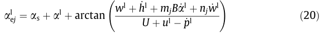
where n_j is introduced to account for the phase lag between the wind fluctuations and the quasi-steady aerodynamic force. The n_j coefficient is obtained as follows:

where G_jw and F_jw are the real and imaginary term, respectively, of the aerodynamic admittance functions of the vertical fluctuations at high reduced velocity for in the preceding equations. It should be noted that this model, using reological transfer functions, is sometimes referred to as the corrected band superposition model [19]. The HNL model retains the advantage of the aerodynamic nonlinearity of the QS model for the high reduced velocity range, and since the unsteady characteristics are distinctive for the low reduced velocity range, the LU model is used to capture the fluid memory effect.

《3.   Application》

3.   Application

In the design procedure of long-span bridges, the erection stage is of particular interest, as the structural system substantially differs from the final form of the structure. The reference object for this study is  a  segment  of  a  multi-span  cable-stayed  bridge  (Fig. 2), erected by the traditional balanced cantilevering method. The aerodynamic models described in Section 2 are applied in order to obtain the structural response due to wind action.

《Fig. 2》

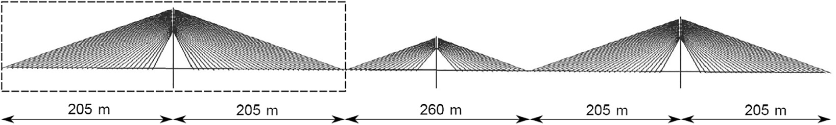
Fig. 2. Reference object: The west tower of a cable-stayed bridge in the erection stage.

《3.1. Structural system》

3.1. Structural system

The two cantilevers on each side of the tower are 205 m long (Fig. 2) with a concrete box section that is B = 33.15 m wide and   H = 4.85 m deep (Fig. 1). The mass and rotational mass are 28.71   t and 2992 t m² per meter, respectively. Fifty-seven  stay  cables are considered in the maximum cantilever stage, with an 8 m distance between the concrete segments. The vertical distance between the tip of the tower  and  the  deck  surface  amounts  to 96 m. Thus, the smallest angle between the  deck and the cables     is 25.4°, while the largest angle is 68°. A total of 15 modes of vibration are used in the analysis, including tower modes. The first lateral, vertical, and torsional modes are given in Fig. 3. In addition, the  natural  frequencies  are  listed  in  Table  S1  in  SI.  The  modal damping ratio is taken as 1% of the critical damping. The inherent property of this type of girder is its high sectional modulus, which results in a rather high structural stiffness compared with light streamlined sections. Taking this into account, the modal properties of the first three deck natural frequencies are somewhat higher than those of flexible cable-supported bridges.

《Fig. 3》

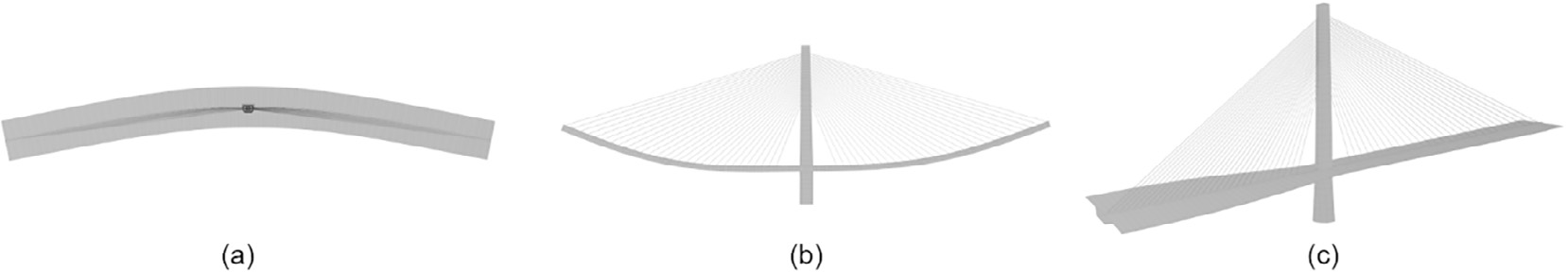
Fig. 3. (a) First lateral (f = 0.401 Hz), (b) vertical (f = 0.444 Hz), and (c) torsional (f = 0.913 Hz) modes of the west tower in the erection stage.

《3.2. Aerodynamic coefficients》

3.2. Aerodynamic coefficients

The static wind coefficients and the flutter derivatives are obtained by utilizing the computationally efficient CFD code VXflow, which is based on the vortex particle method that was developed and validated by Morgenthal [39]. Bluff  box  girders  are usually prone to torsional flutter, and their flutter derivatives are rather irregular and sensitive on the angle of incidence, while the moment static wind coefficient may experience a negative slope, which indicates stall. Looking at  the static  wind  coefficients in Fig. 4, a nearly zero slope is obtained near the positive 6° angle of inclination, which is the first indication of torsional flutter. The flutter derivatives based on the rotational motion are depicted in Fig.  5.  A  particular  point  of  interest  is  the  derivative ,  which  is related to the torsional damping and which changes sign for a positive 3° and 6° angle of incidence, indicating torsional flutter. The flutter  derivatives  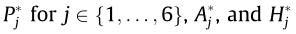  for are considered to be their quasi-steady values [6]. The approximation of Sears’ admittance given in Ref. [40] is used for the lift and moment forces aerodynamic admittance functions. For the drag buffeting component, the admittance is assumed to be unitary.

《Fig. 4》

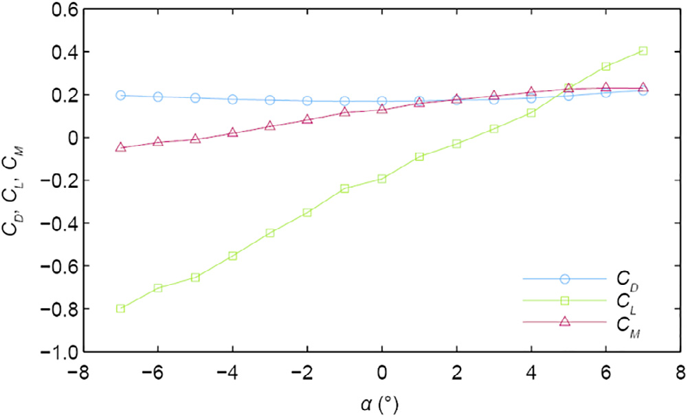
Fig. 4. Static wind coefficients.

《Fig. 5》

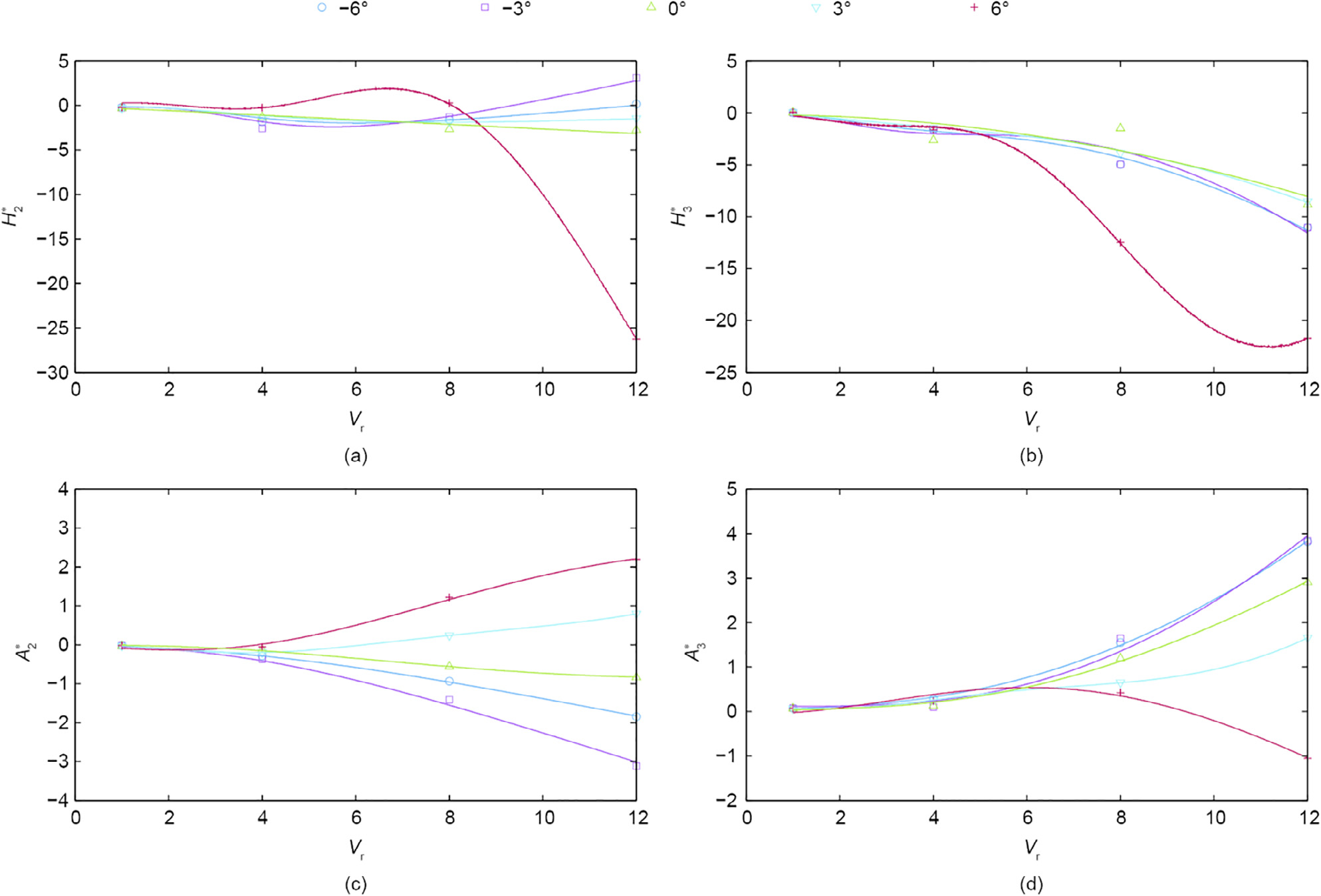
Fig. 5.  Flutter derivatives due to torsional motion for various angles of incidence and their rational approximation (denoted by the line in corresponding color).

In Fig. 6(a), the real and imaginary parts of the Sears’ admittance are given. Two additional aerodynamic states were sufficient for the rational approximation of the admittance. In addition, Fig. 6 (b) gives the phase angle of the admittance transfer function. It can be observed that for  there is a significant change, while for   the  phase  slowly  attenuates.  This  is  important  for  the  n coefficient in the HNL model. Although it is difficult to say at which reduced velocity the phase becomes negligible, n is obtained here based on the interpolation of the admittance at V_r = 15. In the case of experimental complex admittance functions, the phase usually converges  faster.  The  correction  coefficient   ,  which  is  based  on the  flutter  derivatives  in  the  CQS  model  for is  shown in Fig. 7 for Vr = 4. The fluid memory influences the moment forces more than the lift forces in this case, and generally reduces the response. For an angle of incidence that is greater than zero, the effect seems to be noisier than for the negative angles. The joint acceptance considering the higher correlation of the buffeting forces compared with the wind fluctuations is neglected  within this work.

《Fig. 6》

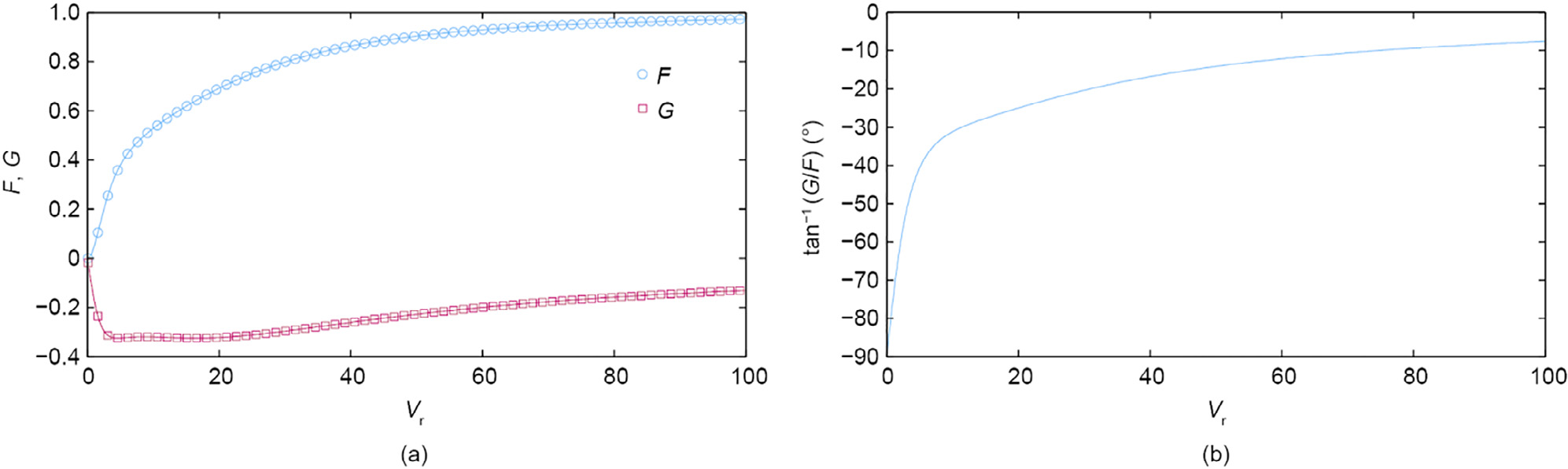
Fig. 6. (a) Real and imaginary parts of the Sears’ aerodynamic admittance and their rational approximation; (b) phase angle between the wind fluctuation and buffeting force.

《Fig. 7》

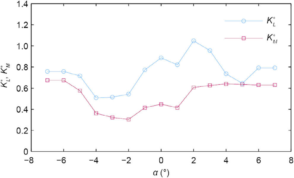
Fig. 7. Correction coefficients for the lift and moment force of the CQS model.

《3.3. Buffeting analysis》

3.3. Buffeting analysis

Turbulent wind fluctuations are applied only to the deck, without the loss of generality. Fluctuating wind time histories are generated for t = 600 s with= 0.01 s for six different wind speeds ranging from 25 m s^_-1 to 75 m s^_-1, using the spectral method described in Ref. [41]. The spectral properties of the fluctuations are based on the von Kárman power spectral density (PSD), as described in Ref. [42]. Two cases are considered: a case with lower turbulence, in which the turbulence intensity is set as I_u = 12% and I_w = 6% for the longitudinal and vertical fluctuations, respectively, and a case with higher turbulence, with I_u = 24% and I_w = 12%. The vertical and longitudinal length scales are set as L_u= 140 m and L_w = 56 m, respectively. The lateral coherence coefficient  is  set  as  8,  using  Davenport’s  coherence  function  [42]. At every wind speed in both turbulent cases, the same time history   is used for all of the models; that is, the input wind fluctuations   are identical.

Fig. 8 depicts the root-mean-square (RMS) from the vertical displacement and rotation for a wind speed of 75 m s—1. The RMS is chosen as a quantity of interest, as the variation in the kinetic energy due to the random generation of wind fluctuations is lower than the peak of the response, since only one realization of the wind time history is utilized. Three main branches can be distinguished in the magnitude of the response. The first of these has  the highest amplitudes for models—that is, the ST and LST models—when the self-excited forces are neglected. The second contains all of the previously described models, without considering the aerodynamic admittance. In the last one, the admittance is introduced for the MQS, CMBM, LU, and HNL models and is denoted by the subscript “A.”

《Fig. 8》

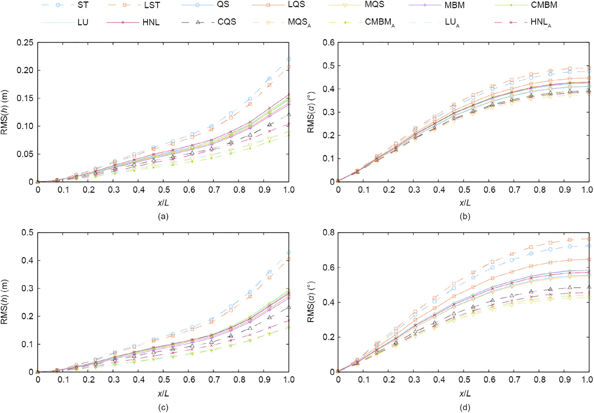
Fig. 8. The RMS of the (a, c) vertical displacements and (b, d) rotation for the case with (a, b) low turbulence (with I_u = 12% and I_w = 6%) and for the case with (c, d) high turbulence (with I_u = 24% and I_w = 12%) for U = 75 m•s^-1. Models considering the aerodynamic admittance are denoted by the subscript “A.”

The branches tend to diverge with the increment of the turbulence intensity, due to the higher influence of the aerodynamic admittance and self-excited forces. This is particularly  true  for  the rotation. In a realistic situation, the aerodynamic admittance differs from the Sears’ function, which would probably reduce its significance for the response.

The influences of the mean wind speed on the tip-displacements of the second and third branch are shown  in  Fig. 9. As the mean wind speed increases, the effect of the fluid memory of the buffeting forces is more influential for the vertical displacements. The trend is similar to that for the rotation; however, it is less pronounced. When comparing the two levels of turbulence intensity, the effect of the aerodynamic admittance is seen to be intensified for the high-turbulence case. In order to study the effects of the assumptions that are implied in each model on the magnitude, phase, and spectral content of the response, a representative part of the time histories is  depicted in  Fig. 10 for U = 75 m s^-1 for the case with high turbulence. The PSDs are shown in Fig. 11. First, the effect of nonlinearity is analyzed without considering the self-excited forces. The nonlinearity included in the ST model increases the response in the vertical DOF, while the rotation is reduced. Since no additional phase lag is introduced in these models, the nonlinearity only affects the amplitudes. By comparing the LST and LU models, the influence of the self-excited forces on the response can be studied. Introducing unsteady aerodynamic damping and stiffness reduces the response and introduces a small lag. The effect is more severe for the vertical DOF (Fig. 9). The difference in the PSD of these two models occurs mainly at the peaks for the first vertical and torsional natural frequency.

《Fig. 9》

Fig. 9. The RMS of the cantilever tip (a, c) vertical displacements and (b, d) rotation for the case (a, b) with low turbulence (with I_u = 12% and I_w = 6%) and for the case (c, d) with high turbulence (with I_u = 24% and I_w = 12%). Models considering the aerodynamic admittance are denoted by the subscript ‘‘A.”

《Fig. 10》

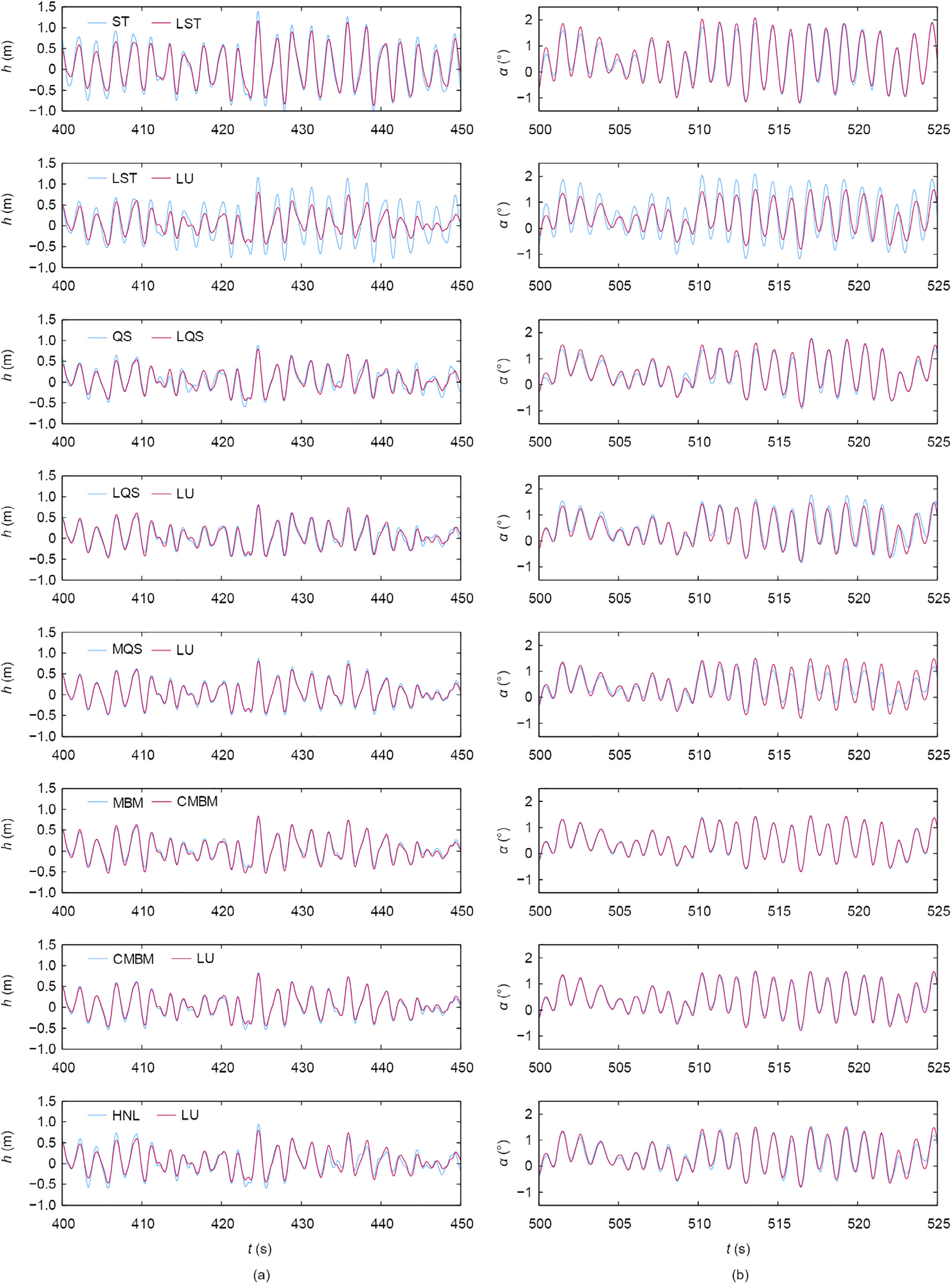
Fig. 10. Representative sample time histories of the cantilever tip (a) vertical displacements and (b) rotation for the case with high turbulence (with I_u = 24% and I_w = 12%) at U = 75 m•s^-1. Models considering the aerodynamic admittance are denoted by the subscript ‘‘A.”

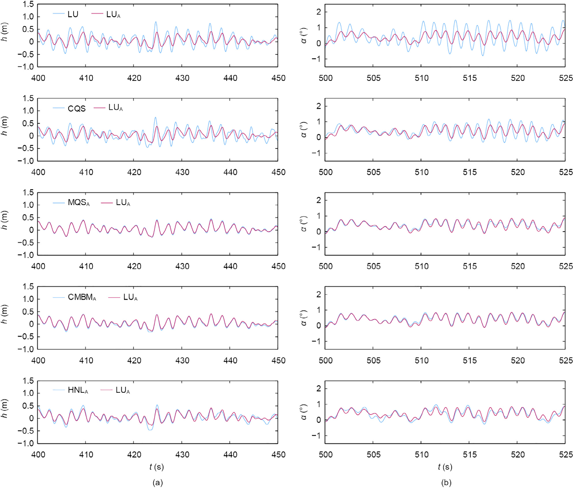
Fig. 10 (continued)

《Fig. 11》

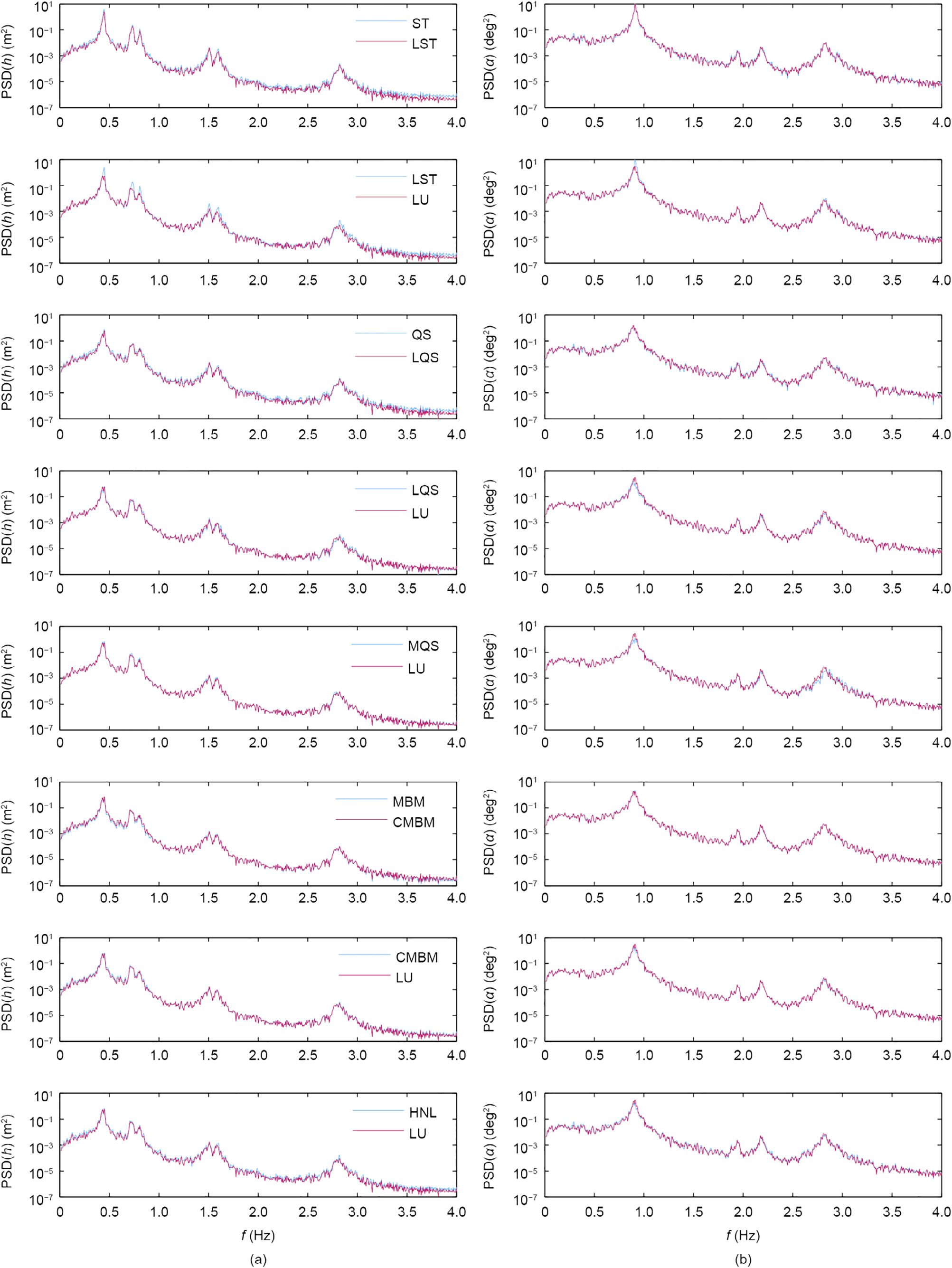
Fig. 11. The PSD of the cantilever tip (a) vertical displacements and (b) rotation for the case with high turbulence (with I_u = 24% and I_w = 12%) at U = 75 m•s^-1. Models considering the aerodynamic admittance are denoted by the subscript ‘‘A.”

Fig. 11 (continued)

The second branch is constituted of the models that consider the self-excited forces and neglect the aerodynamic admittance— that is, the QS, LQS, MQS, MBM, CMBM, LU, and HNL models. Before examining the second branch, it should be noted that the difference in the RMS between the  lowest  and  the  highest  response for the case with low turbulence is 11.6% and 8.28% for the vertical displacements and rotation, respectively. In the case with high turbulence, the difference is 10.1% and 15.2% for the vertical and rotational DOF, respectively. The larger discrepancy in the rotation for the high-turbulence case is attributed to the LQS model. The observations for this branch are mainly based on Figs. 8 and 9, since for such small differences, it is difficult to select a representative time history and draw a conclusion based on it and on the corresponding PSDs. Nevertheless, the time histories and PSDs are depicted for the sake of consistency.

The discrepancies between the QS and LQS models are due to the aerodynamic nonlinearity in the QS model, considering the quasi-steady self-excited forces. The influence of the aerodynamic nonlinearity or the vertical DOF is small compared with the case without self-excited forces, although it is still significant for the rotation in the high-turbulence case. To study the effect of the fluid memory of the self-excited forces on the response, the responses obtained from the LQS and LU models are analyzed. Looking at Figs. 8 and 9, it can be observed that for the vertical DOF, the response is slightly higher for the LU model, while the torsional response is increased for the LQS model. In general, the fluid memory should reduce the response of the deck; however, here the differences are small and may originate from the ambiguity of the aerodynamic center in the LQS model. Looking at the influence of the averaged fluid memory of the self-excited forces as considered in the MQS model, in contrast to the full fluid memory included in the LU model, it can be observed that there are no significant differences in the response for the vertical DOF. However, for the MQS model, the torsional response is underestimated to a small extent; this can be also observed in the PSD. By comparing the MBM and CMBM models, the effect of the aerodynamic coupling can be studied. Excluding the aerodynamic coupling, the MBM model underestimates the vertical response by 6.5% and 8% and the rotation by 1.7% and 0.7% for the cases of low and high turbulence, respectively. The resemblance between the LU and CMBM models leads to the conclusion that interpolating the flutter derivatives at the complex frequencies instead of considering the broad band frequency content has no significant influence on the response for both DOFs.

The impact of the aerodynamic nonlinearity on the lowfrequency response and the influence of the fluid memory of the self-excited force in the low reduced-frequency range of the oscillation are investigated by comparing the responses from the LU and HNL models. A minor difference is observed in the vertical component for the low-turbulence case.

The significance of the aerodynamic admittance on the  response is substantial in this case. An examination of the response from the LU model with and without admittance reveals a change in the amplitude and phase in the time histories. In the PSDs, the overestimation of the LU model is higher for the high-frequency components.

This result is in line with the underlying physics of bluff body aerodynamics, as gusts with small wavelengths compared  with  the deck width have less-significant influence on the buffeting forces. The incorporated averaged fluid memory in the CQS model does not entirely unveil the effect of the rise time of the buffeting and self-excited forces. Compared with the LU model that considers the aerodynamic admittance, there is a discrepancy in the phase and an amplitude amplification in the response, especially  in the low-frequency component. It can be  argued  that  this  is  due to the aerodynamic nonlinearity.  However,  the  significance of the aerodynamic nonlinearity is expected to be lower, judging from the performance of the QS and LQS models. For the MQS model that includes the aerodynamic admittance, and for which the fluid memory in the buffeting forces is included by means of Eq. (16), no appreciable differences in the vertical response are noted with respect to the LU model for the high-turbulence case. The vertical response in the low-turbulence case and the rotation in both cases, however, are underestimated for the MQS model. This result is attributed to the averaged fluid memory in the selfexcited forces for the case in which the buffeting and self-excited forces act simultaneously. Similar results for the response are obtained for the CMBM and LU models when both consider the aerodynamic admittance, thereby proving the validity of the method for the computation of buffeting forces that was presented in Section 2.4.1. An interesting point arises when the responses for the HNL and LU models are compared when both models consider the aerodynamic admittance. The RMS of the vertical displacements is generally higher for the HNL model. Although this is usually the case for flexible bridge decks due to the static nonlinearity,in this case, it is associated with the chosen cut-off frequency of 0.3 Hz between the lowand high-frequency components of the wind fluctuations. Looking at the PSD of the response, it is observed that the main distinction is in the low-frequency component as a result of neglecting the aerodynamic admittance in this range, rather than the aerodynamic nonlinearity. There have been several studies on the choice of the cut-off frequency. In Ref. [18], the threshold is taken as the first oscillation frequency, whereas in Ref. [19], it is chosen based on the reduced velocity—that is, at V_r ≥15. Wu and Kareem [29] conducted a parametric study and concluded that the increase of the response may arise from the frequency content of the effective angle of attack, rather than the amplitude. It can be argued that in this case, the cut-off frequency is chosen to be rather higher than the reduced velocity range in which the quasi-state assumption holds true, which explains the higher amplitudes in the low-frequency content. However, further examination is required on this account, and is beyond the scope of this study.

In Section 2.4.1, an alternative approach is presented for the computation of the buffeting forces including the aerodynamic admittance. In order to test its applicability, the lift force acting on the cantilever tip for the high-turbulence case is compared with the standard linear unsteady formulation. In Fig. 12, the time history of the normalized lift force is presented, computed without and with admittance. In the latter case, two methods were used: the standard method, based on rational approximation, and the introduced method, based on the inverse FFT. The time histories of the normalized lift force for the two methods including the aerodynamic admittance correspond well, except for the initial  part (for t≈ 0–3 s), in which the transient part of the lift force is considered by means of the standard method using rational approximation. Although the rise time depends on the properties of the aerodynamic admittance, this part is usually short compared with the full length of the force time history. The relative difference in RMS for t = 600 s is less than 0.2%.

《Fig. 12》

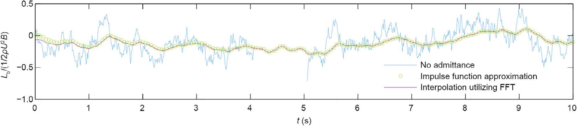
Fig. 12. Representative sample time histories of the cantilever tip vertical buffeting force for the case with high turbulence (with I_u = 24% and I_w = 12%) at U = 75 m•s^-1. The unsteady forces are computed using the rational approximation of the admittance by impulse functions (Eq. (S10) in SI) and the presented method using the FFT (Eq. (16)).

《3.4. Flutter analysis》

3.4. Flutter analysis

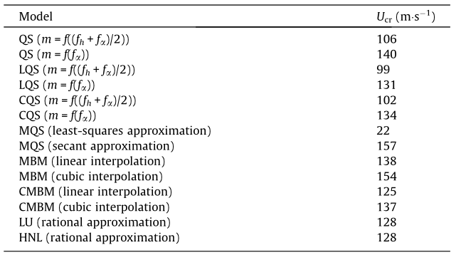
A stability check during the cantilever erection stage for cablestayed bridges presents a particular issue, as the torsional stiffness of the deck is usually lower than that in the in-service condition. As discussed briefly in Section 3.2, this cross-section is prone to torsional flutter if there is a change in the angle of the incident wind, which  can  be   easily  identified  by  the  changing  sign  of   the   Am2 derivative (Fig. 13) that is related to the torsional damping of the system. The flutter analysis is performed for uniform flow at a 6°angle of incidence, since the section is stable at 0° for velocities up to 175 m s^-1. Checking the flutter limit for higher wind speeds would have required extrapolation of the flutter derivatives.  In Fig. 14, an example of the time history is shown for the LU model below and at the critical wind speed. Some of the nonlinear models, such as the QS and CQS models, can exhibit limit cycle oscillations; however, their time histories are not presented here for the sake of brevity. Further information on the flutter and post-flutter regime can be found in Ref. [29]; in this paper, only the critical flutter limit is addressed. Table 1 provides the critical flutter velocities for the selected models. The reference case for the flutter analysis is the CMBM model, since it represents a multi-mode frequencydomain analysis that has been experimentally validated on several occasions (see e.g., Ref. [43]). The critical limit for the QS, CQS, and LQS models is calculated for different values of the aerodynamic center. In the case of these models, torsional instability in bridge aerodynamics occurs if the aerodynamic center is positioned between the trailing edge and the stiffness center; that is, mα > 0.

《Fig. 13》

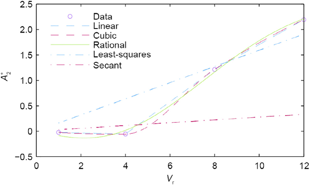
Fig.  13.    derivative:   linear   and   cubic   interpolation   for   the   MBM   and   CMBM models; rational approximation for the LU and HNL models;  least-squares and secant approximation for the MQS model.

《Table 1》

Table 1 Critical flutter velocities for wind at a 6° angle of incidence.

《Fig. 14》

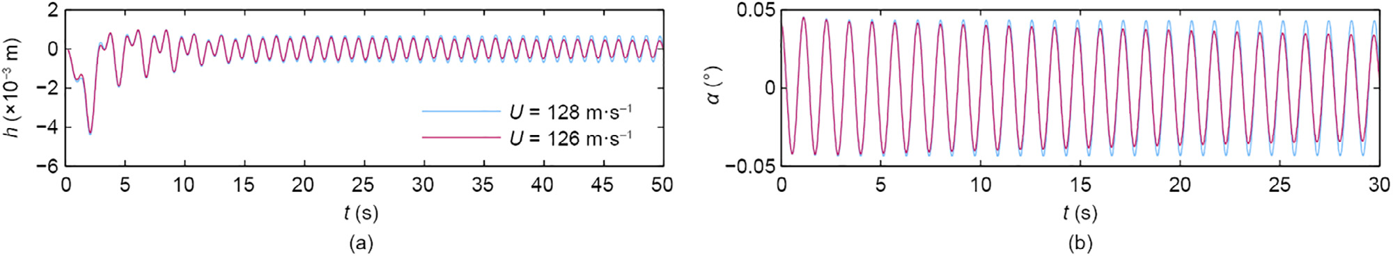
Fig. 14.  Time histories of the (a) vertical displacement and (b) rotation under laminar flow of the LU model at critical flutter velocity (U = 128 m•s^-1) and below flutter   velocity (U = 126 m•s^-1) at a 6° angle of incidence.

For streamlined bridge decks, this coefficient is commonly set as   0.25,  which  ensures  no  occurrence  of  torsional  flutter;  or,  it  is obtained from the flutter derivatives (Eq. (11)) for high reduced velocity. Flutter cannot occur in this case by choosing Vr ≥ 12 at a 6° static angle of incidence. Although the value of is negative, is negative as well (Fig. 5), resulting in a positive value for the aerodynamic  center.  Negative  values  for  Am3    rarely  occur,  and  at  high reduced velocities,  the  quasi-steady  values  indicate  stall;  that  is,    However,  some  studies  have  reported  a  negative  value for ,  such  as for  the Tacoma Narrows  Bridge  section reported in Ref. [44], or for the Deer  Isle-Sedgewick Bridge section cited in Ref. [13]. Therefore, the assumption of selecting the aerodynamic center at high reduced velocities may be challenged for bluff bridge decks that are prone to torsional flutter. At present, it is not clear whether this is the same phenomenon that was identified as the velocity-restricted torsional flutter in the experimental study for rectangular cylinders in Ref. [45]. Flutter  analysis  is  conducted for two cases with respect to the aerodynamic center. In the first case, the aerodynamic center is based on the reduced velocity for the central frequency of oscillation m = f((f_h + f_α)/2), while in the second case, the torsional frequency is used for the determination of the aerodynamic center m = f(f_α). For these values, the coefficient is  still  in  the  positive  range.  The  critical  velocity  for  the  LQS model with  the aerodynamic center  obtained using  the   torsional frequency is comparable to the critical velocity obtained using the CMBM model. This makes sense because the oscillation is driven by the pitching motion and the coupling effects have minor influence. The underestimation of 4.4% of Ucr for the LQS model as compared with the CMBM model can be attributed either to the fluid memory of the self-excited forces or to the ambiguity of the aerodynamic center; the latter explanation is more plausible. The influence of the aerodynamic nonlinearity included in the QS model increased the flutter velocity by 6.4%. By including the averaged fluid memory for the CQS model, the flutter limit is reduced by 4.3% compared with the flutter limit obtained using the QS model. It is  worth mentioning that the models in which the aerodynamic damping is based on the  aerodynamic  center  may  overestimate or underestimate the flutter velocity by a relatively large margin; therefore, such models are generally not used for the flutter analysis.

 As a result of the nearly quadratic shape of the Am2  derivative, the critical flutter velocity obtained using the linear least-squares approximation for the MQS model is underestimated significantly. The accuracy of the MQS model is generally good for linear trends for the velocity-related and quadratic trends for the displacementrelated flutter derivatives. For different trends than this, the secant approximation is used for the reduced velocity of interest, as pointed  out  in  Ref.  [16].  Utilizing  the  secant  approximation for  Am2 with respect to the torsional frequency, the  analysis  with  the  MQS model yielded an overestimation of the  flutter  limit  by  14.6% compared with the limit obtained using the CMBM model with cubic interpolation. In the case of pure torsional flutter, the MBM and CMBM models would result in the same critical velocity. However, the instability threshold for the MBM model was under-

estimated by 12.4% and 10.4% in the case of cubic and linear interpolation of the flutter derivatives, respectively, due to the effect of the aerodynamic coupling. Theoretically, the CMBM and LU models should result in an identical flutter limit, since the CMBM model has the same complex modal properties as the full frequencyindependent system (as noted in Ref. [17]). Nonetheless, the critical flutter velocities are slightly different. This is a consequence of the  goodness-of-fit  of  the  Am2    derivative,  which  is  observable  in Fig. 13. In fact, the critical velocity for the LU model using rational approximation is somewhere in between the Ucr values that are obtained using linear and cubic interpolation,  respectively,  for  the CMBM model. The effect of the uncertainty in the interpolation or approximation of the flutter derivatives is expected to be reduced by increasing the number of data points. The flutter is gov-

erned by the linear unsteady part in the HNL model. Since the flutter derivatives at 6° are used for both the LU and HNL models, the instability threshold is identical. In general, the results may differ, as the HNL model is linearized at the angle obtained using nonlinear aerostatic analysis, or if the response is governed by the quasisteady part.

《4.   Summary and conclusions》

4.   Summary and conclusions

Various models for buffeting analysis have been studied here, and the effects of their implied assumptions have been quantified with respect to the dynamic response of a particular bridge in the erection stage. The influence of the self-excited forces and the aerodynamic admittance on the response appeared to be most significant in the design velocity ranges, especially for the highturbulence case. By increasing the complexity, the aerodynamic models can account for more phenomena occurring in the FSI. However, the influence of the fluid memory in the self-exited forces, aerodynamic nonlinearity, and even aerodynamic coupling appeared to be less significant for the aerodynamic response for the selected case.

An initial assessment in the erection condition for less-severe wind conditions could be performed with less-complex models such as the MQS model including the aerodynamic admittance, given sufficient care for the goodness-of-fit of the derivatives. Nevertheless, more complex models, such as the LU, CMBM, or HNL models, should be utilized for the final checks in the design process.

Furthermore, a method for the inclusion of the aerodynamic admittance in the CMBM model was presented here based on the principles of the response of a stable linear system, utilizing the Fourier transform. The results of the buffeting force using this method agreed well with the standard method utilizing the impulse function formulation. The rational approximation using the presented method is avoided. It should be noted that the method can also be used in the LU model without the loss of generality. Within the present study, the RMS of the response is taken as a quantity of interest, since it can be correlated to the kinetic energy. Further statistical studies are warranted on the extreme values of the response, as there is no direct relationship between the RMS and the peak for the nonlinear models.

Flutter analysis was conducted for mean wind velocity at a 6° angle of incidence. The aerodynamic center in the QS-based models came under special consideration. The analysis showed that in the case of torsional-driven flutter, the aerodynamic center chosen with respect to the torsional frequency of oscillation provides better estimates corresponding to the standard frequency-domain flutter analysis. Accounting for the aerodynamic coupling resulted in a reduction of the flutter velocity of approximately 10% for the particular case study. The interpolation or approximation method of the flutter derivatives was demonstrated to have an effect on  the on-set flutter velocity. Further studies considering the influence of the data quality of the aerodynamic derivatives on the buffeting response are of interest. In conclusion, the model choice is highly dependent on the case study, and it is in the designers’ interest to evaluate various models based on their assumptions and on the available aerodynamic properties in order to obtain a reliable estimate.

《Acknowledgements》

Acknowledgements

This research is supported by the German Research Foundation (DFG) via Research Training Group ‘‘Evaluation of Coupled Numerical and Experimental Partial Models in Structural Engineering (GRK 1462),” which is gratefully acknowledged by the authors.

《Compliance with ethics guidelines》

Compliance with ethics guidelines

Igor Kavrakov and Guido Morgenthal declare that they have no conflict of interest or financial conflicts to disclose.

《Appendix A. Supplementary data》

Appendix A. Supplementary data

Supplementary data associated with this article can be found, in the online version, at https://doi.org/10.1016/j.eng.2017.11.008.