

1. Introduction
As an accompanying phenomenon of rock mass deformation, crack initiation, and crack propagation, a microseismic event is an earthquake with a magnitude lower than 3.0, and with weaker energy and a lower signal-to-noise ratio (SNR) than large natural earthquakes. Microseismic monitoring is a record of the temporal and spatial features of microseismic phenomena [1].
In the early 1960s, researchers from South Africa and the United States began to study and utilize microseismic techniques to monitor rockburst location. Since the mid-1980s, over 20 rockburst-prone mines in Canada have been installed with micro-seismic systems so that severe rockburst disaster can be routinely monitored [2]. Luo and Hatherly [3] applied this technique to undertake microseismic monitoring at two long-wall mines. Their work also concentrated on constructing the patterns of induced fracturing in the roof and floor. Rutledge et al. [4] successfully conducted a hydraulic fracture operation in the Cotton Valley gas field in East Texas, USA, in the same year. The typical substation structure of a microseismic monitoring system is shown in Fig. 1.
《Fig.1》

Fig. 1. Structure of a microseismic monitoring system in a mine. GPS: global position system.
Locating the source of a microseismic event in a mine—that is, determining exactly where and when the shocks originated in three-dimensional (3D) space—remains a complicated undertaking, as it is influenced by multiple factors. Microseismic source location is the essential factor in microseismic monitoring technology, and the precision of microseismic source location will greatly influence the application of the microseismic technique.
Most microseismic phases are body waves, which are consid-ered to propagate in unbounded homogeneous media in mine-related microseismic events. Both P and S waves can propagate in any direction. Research into locating microseismic sources can be based on existing research on locating the sources of natural seismological events, since microseismic signals have a similar focal mechanism and signal characteristics to natural earthquake signals. However, the triaxial sensor localization and geometric mapping methods (including the Ishikawa Nori method, a virtual method, a intersection method, and a midline method) that are used in seismic source location are not suitable for microseismic source location in a mine. The triaxial sensor method can be carried out from a single sensor location, and can be applied to seismic source location in a situation with fewer measuring points. Although this low-cost method provides stress wave characteristics at the measuring point, its weakness is that material structures and properties strongly affect signal amplitude [5]. The Ishikawa Nori method can be used to determine the position of an earth-quake based on the velocity of seismic wave propagation, V, and the first arrival times of the direct P wave and the S wave (P;S) [6]. There are three main methods to determine time and space parameters near an earthquake: the Wadachi, Ishikawa, and Takahashi methods. Of these methods, the Wadachi method is based on the source trajectory method, in which the difference in the first arrival times of the P wave and the S wave as observed by more than four stations, is used to determine the position of the hypocenter.
Both the P and S wave arrival times are taken into consideration in the seismic source-locating methods listed above. However, because the source is too close to the sensor in microseismic monitoring in a mine, most of the signal S waves detected by microseismic monitoring are not obvious. In addition, direct S waves are easily disturbed by the subsequent coda wave of the P waves. Taking these factors into account, the P wave signal may be submerged by all kinds of underground noises, given the weak signal energy. Only the S wave signal, which has stronger energy, can be received. Therefore, methods that are based on P and S waves are limited in their application to locating microseismic sources in a mine.
A source location method based on seismic arrival time can be applied to the source location of earthquakes, microseisms in a mine, and acoustic emissions. In the 20th century, numerous classical source location methods—such as the Geiger iterative localization algorithm; the Inglada method, which serves as a non-iterative lin-ear source location method; and the double-difference method— were proposed for earthquake source location. With the develop-ment of microseismic monitoring technology, source localization methods for microseismic monitoring began to be proposed starting in the early 1960s, and a source location method was proposed by the researchers in the United States Bureau of Mines in the early 1970s. At the end of the 1980s, the simplex method of microseismic source location was introduced [5,7]. Most of these location meth-ods are still used for microseismic source location.
Classical location methods based on arrival time can easily be affected by the precision of the arrival time picking and by the wave velocity model, leading to low precision in location results. The abovementioned classical methods have been improved, and optimal combinations of multiple methods have been proposed in the 21st century. Meanwhile, several new microseismic source location methods involving time-reversal imaging and interferometric imaging have been put forward, and are expected to be applied to microseismic source location through optimize parameters.
Our intention is to determine the key factors involved in reduc-ing location errors and increasing the reliability and precision of location results by analyzing existing research on microseismic source location methods in mines since the year 2000. Based on the monitoring purpose and the characteristics of the monitoring system, we propose an optimum method to realize the high-precision location of microseismic events in mines.
《2. Research development on microseismic source location in mines》2. Research development on microseismic source location in mines
The least-squares method [8] and the Newton iteration method [9] have been used to identify the source location of microseisms in a mine. However, the weak and low SNR of microseismic signals results in problems such as an inaccurate first arrival time and inefficient identification of the location of the hypocenter. To address these problems, conventional source location methods for mine’s microseisms have been constantly optimized and improved since the year 2000. Some representative methods are described below.
《2.1. Combined location method: Linear and Geiger methods》2.1. Combined location method: Linear and Geiger methods
A combined location method that involves both the linear location method and the Geiger location method has been proposed [10]. Preliminary microseism location identification is carried out using the linear method; the obtained solution is then used as the iterative initial value of the Geiger location method in order to calculate the final position. Field measurement results were presented in this study, which demonstrated the improvement in the precision of the source location.
《2.2. Combined location method: Least-squares and Geiger methods》2.2. Combined location method: Least-squares and Geiger methods
Kang et al. [11] utilized the least-squares method to provide the initial iteration point, and then calculated the source position iteratively using the Geiger algorithm. Combining the least-squares method with the Geiger algorithm resulted in an increase of the source calculation speed.
《2.3. Combined microseismic event location method》2.3. Combined microseismic event location method
Although traditional location methods identify single events independently, Poliannikov et al. [12] considered it to be advanta-geous to locate multiple seismic events with uncertain velocity simultaneously. A combined method can be used to update the locations of all events simultaneously. In the presence of velocity uncertainty and signal noise, this framework for the combined location of microseismic events reduces the error in estimated fracture size.
《2.4. Optimization of relative location method》2.4. Optimization of relative location method
Got and Okubo [13] proposed a modified master event method that simply uses a velocity model to calculate the travel time difference, thus greatly reducing the influence of the velocity model on the location precision. A master–slave relation is established between events of known source parameters and those of unknown source parameters, and a travel time circle is established around the master event so that the arrival time of the slave event is completely avoided. Grechka et al. [14] proposed a multimaster relative event location method. Based on the constructed layered velocity model, different weights are assigned to different master events in order to locate the same event, which is eventually located by using the adjacent master event.
Castellanos and Van der Baan [15] proposed a cross-correlation method to detect microseismic events with similar waveforms; the waveform similarity represents the appropriate weighting coefficients. The double-difference algorithm, which is a relative location method, can be used to relocate microseismic events when they originate in the same source region with identical source mechanisms during a one-month period. Picking errors are major sources of event relocation, but these can be corrected through the cross-correlation method [16]. The assumption of a homogeneous velocity model greatly simplifies velocity model building. Ref. [16] plugs the weight that is based on event similarity into the double-difference method. The result is then compared to the original method that weight coefficient is based on inter-event distance developed by Waldhauser.
Chen et al. [17] developed a new seismic tomography method, using back azimuth constrained double-difference seismic tomography, which results in more accurate relocation than the conventional grid search location method.
《2.5. Location method without pre-measured velocity》2.5. Location method without pre-measured velocity
Dong et al. [18] proposed three methods for microseismic source location without pre-measured velocity. Of these methods, onsite data revealed that the time-difference (TD) method has bet-ter location precision and stability. With this method, only the sensor coordinates and time differences are needed. The TD method takes the velocity of the wave as an unknown quantity and solves it with the source coordinate; it does not need to fit the time of earthquake occurrence. Thus (x0, y0, z0, c) should minimize Q(x0, y0, z0, c); that is

where (x0, y0, z0) is the source coordinate; c is velocity; i and j are the sensor numbers; n is the total number of the sensors; Lcj is the distance between the ith sensor and source; Lcj is the distance between the jth sensor and source;  is the arrival time difference regression value between ti and tj; ti is the arrival time of the ith sensor; and tj is the arrival time of the jth sensor.
However, when the position of the hypocenter and the velocity of the wave are coupled together to inverse, it is unfavorable for inversion of microseismic source position.
《2.6. Location method without arrival time picking》2.6. Location method without arrival time picking
Kao and Shan [19] introduced a new method, the source-scanning algorithm, to image the distribution of seismic sources. The concept behind this new algorithm is based on looking for possible microseismic sources in both time and space. This method exploits waveform information, including amplitudes and arrival time, from an array of seismic stations, in order to determine whether or not a seismic source is present at a particular time and position. By systematically scanning through a range of trial source positions and origin times, it is possible to recover the entire distribution and sequence of seismic sources without need-ing to pick the arrival time of seismic phases accurately or to calculate synthetic seismograms.
He [20] proposed a method to retrieve the microseismic source by using multi-level three-component data. First, the orientation angle of the horizontal geophones needs to be determined. Next, the travel time of the direct P wave is calculated from every geo-phone point in 3D space. At any given moment, the energy and maximum of the three components in the time window are obtained along the first arrival direction of the longitudinal wave, and the inversion of the hypocenter position is carried out. This method solves the problem of multiple solutions without picking an arrival time; however, it is greatly influenced by the wave velocity.
Kinscher et al. [21] presented two probabilistic methods that provide a powerful tool to automatically assess the spatiotemporal characteristics of swarming sequences. Both methods take advantage of strong attenuation effects and significantly polarized P wave energies at higher frequencies.
These methods use combined parameter optimization, or abandon a certain parameter, in order to optimize the traditional methods. However, monitoring system performance, geophone distribution, velocity model, or first arrival time-picking errors have an impact on each method. The huge location errors that still exist under the monitoring area are complicated, and basic data cannot be acquired accurately.
《3. Factors influencing microseismic source location》3. Factors influencing microseismic source location
Microseismic source location procedures are usually carried out in a very complex environment. Many factors can affect the precision of source location, such as the distribution of seismic stations, the velocity models, and the accuracy of the arrival time picking [22]. In addition, it is extremely difficult to establish an accurate velocity model due to influencing factors such as unpredictable distribution of rock stratum, rock anisotropy, and sudden changes of wave velocity between rock layers. In addition, given the randomness and uncertainty in the propagation of shock waves, interpretation of the communication process still needs further improvement. The microseismic signal is a wideband signal, which leads to difficulty in filtering noise, even though microseismic signals in lower SNR. Thus, if these problems cannot be solved, it is difficult to achieve high-precision locating by means of an inversion location method based on wave velocity and travel time.
Next, we discuss source location factors and response measures.
《3.1. Geophone distribution》3.1. Geophone distribution
The spatial distribution of the microseismic geophones is a key link in identifying the location of the hypocenter, as the distribution of different monitoring stations has different effects on location precision. One of the most important research findings in microseismic monitoring technology is the need to study the distribution scheme of microseismic geophones, which can improve the precision and reliability of seismic source location.
When optimizing microseismic geophone distribution, one should refer to theories on the optimum distribution of a seismic network. These theories include the calculation of network monitoring capability based on the Monte Carlo algorithm [23] and the design of a microseismic network based on degree of seismic danger (D value) and concentrative degree of seismic-spacial (C value) optimum design theory [24].
Based on the theory of D-optimal design, Gong et al. [25] studied the optimal configuration of a seismological network. Guided by the principle of D-optimal design, a low-cost design for a microseismic network for a coal mine can be quickly determined using a genetic algorithm.
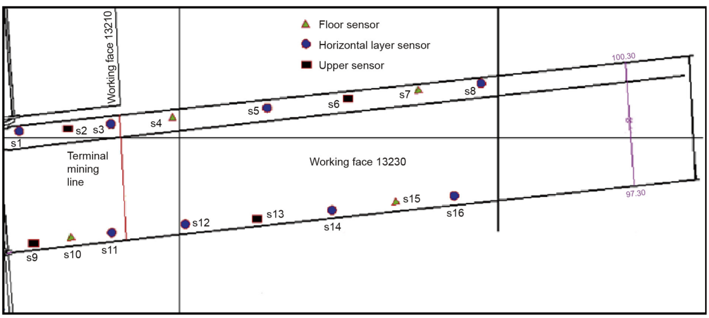
The theory of D-optimal design holds that the optimization of geophone station position depends on the source parameter covariance matrix. Based on the theory of D-optimal design, Gao et al. [26] introduced the probability of occurrence of a microseismic event, the importance of regional monitoring, network deployment feasibility, and other factors to build the objective function; they then established an optimal plan for a microseismic monitoring network in a phosphate ore mine. The microseismic monitoring network that consists of several geophones in a mine working face is shown in Fig. 2.
《Fig.2》

Fig. 2. Arrangement of microseismic geophones in a mine working face (unit: m)
《3.2. First arrival time picking》3.2. First arrival time picking
The influence of several factors, such as the weak radiation energy of microseismic signals in a mine, the high noise level in underground coal mines, and low SNR, greatly increase time-picking errors. Large time-picking errors will occur when extra data are present in the observations. Faced with this problem, Anderson [27] was the first to use the method of discarding special data in order to process data so as to improve the precision of the solution.
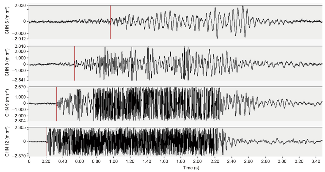
The automatic picking of first arrival time based on Allen automatic picking algorithm (short-term average to long-term average (STA/LTA)) is shown in Fig. 3. With the improvement to the STA/ LTA, Li et al. [28] proposed a microseismic signal that was suitable for the project scale, as well as an Allen coupled with Bear algorithm of the P wave first arrival automatic identification with the introduction of the Bear weighted factor and characteristic function. In this way, the accuracy rate of the first P wave arrival time was improved, albeit only to 73.51%.
《Fig.3》

Fig. 3. Automatic picking of first arrival time at different noise levels. CHN: channel.
To overcome the large picking errors contained in the arrival time picking, Li et al. [29] proposed the virtual field optimization method (VFOM). The results of numerical examples and onsite blasts demonstrate that the VFOM is capable of locating local microseismic and acoustic sources.
Taking into consideration the STA/LTA method and polarization analysis, Song and Feng [30] designed a method for the automatic identification of the valid events of microseismic monitoring data. The valid events of microseisms were identified, followed by the stacked location aimed at identifying events.
《3.3. Velocity model》
3.3. Velocity model
The precision of a microseismic event location is mainly affected by the velocity model hypothesis of rock mass. It is generally assumed that the rock mass has the same elastic modulus properties throughout; thus, a single velocity model is adopted. The uncertainty of the actual rock mass velocity model and the neglect of media anisotropy will lead to systematic unacceptable source localization errors. Therefore, it is not possible to simply use the direct wave hypothesis to determine the propagation of microseismic waves.
A ray-tracing algorithm is used to deal with microseismic events by designing a scientific layered wave velocity model to simulate direct wave and refraction wave propagation. Belayouni et al. [31] developed a ray-tracing algorithm capable of computing the travel time and polarization of direct, refracted, and reflected waves in an assumed layered velocity model in order to locate the source. The algorithm was then applied to handle the real data-set of Cotton Valley, where reflections could be seen for strong events due to the high-velocity contrasts. Compared with a case when only direct wave were utilized, the location precision was improved and the location uncertainty was significantly reduced when using both direct wave and refraction wave.
A single velocity model cannot be acceptably applied to a complex rock mass in the field of mine engineering; it is necessary to build a complex rock mass velocity model, according to the characteristics of the engineering site. Aiming at rock masses with complex partitioned velocities or voids filled with air in actual engineering situations, the multi-stencils fast-marching (MSFM) method was introduced to calculate the travel time of the first arrival wave [32]. The first arrival travel time is calculated by the MSFM algorithm from the origin to the rest of the nodes; the ray path can then be calculated by using the shortest path ray tracing from Dijkstra’s algorithm. The study concludes that the MSFM is very valuable for application as a forward method.
Collins et al. [33] provided a velocity model that accounts for multiple complex-shaped geological units, each with its own properties. This velocity model can be configured to contain space that may be air-filled, brine-filled, or cement paste backfilled. Van Dok et al. [34] proposed the anisotropy parameters that should be acquired during a microseismic monitoring project. These parameters can and should be included in the final velocity model in order to produce more accurate event locations. Michael and Richard [35] performed microseismic event location precision enhancement using anisotropic velocity models. Eisner et al. [36] found that the largest uncertainty in surface monitoring is in the vertical position, due to the use of only a single phase in the estimation of the event location. In surface monitoring results, the lateral position is estimated robustly and is not sensitive to the velocity model.
An error of 5% in the velocity model will cause a large location error. The application of an isotropic velocity model to the actual anisotropic structure will lead to unrealistic speed values. There-fore, the construction of a velocity model must take into account the anisotropy of the rock mass. In addition, the strata structure in the area of the mine under microseismic monitoring tends to be affected by movement of rock during mining procedures, which influences the arrival time and the propagation direction of the microseisms; thus, time and space changes must be considered. Therefore, the velocity model should be evaluated according to the microseismic data. In Ref. [37], the velocity model was updated using the image domain waveform tomography method.
Gesret et al. [38] proposed a new Bayesian formulation that integrates a proper velocity model into the formulation of the probabilistic earthquake location. They propagate the velocity model uncertainties to the seismic event location in a probabilistic framework, which helps to obtain more reliable source locations.
Ge and Kaiser [22] proposed an event-based dynamic velocity model. P, S, and erroneous waves can be detected through first arrival time picking. Its criteria are the sequence and the arrival time difference of the signal from each channel. After using an arrival time difference analysis to assess the position of the two sensors, the observations of the two sensors must be satisfied:

where ti and tj are the arrival time picking of the two sensors, respectively; 2cij is the distance between the two sensors; and vp is the P wave velocity. If the arrival time picking of a certain channel satisfies this equation, then the signal of this channel must be a P wave; otherwise, it is an S wave or an erroneous wave. ti is usually taken as the picking of the arrival time from the first channel that receives the signal [39].
《4. Prospects》4. Prospects
Although considerable efforts have been put into improving the accuracy of first arrival time-picking technology in order to establish a scientific wave velocity model, in most cases, the model is limited by the rock anisotropic medium, the performance of the monitoring instruments, and other factors. The arrival-picking error and velocity model error are still very large, and the results of mine-related microseism locations that are obtained by source location methods based on arrival time are unavailable. Therefore, it is imperative to develop new methods to improve the location precision of microseismic sources.
《4.1. Time-reversal imaging technique》4.1. Time-reversal imaging technique
Xu et al. [40] proposed a new location method called time-reversal imaging, which is based on wave equations instead of travel time. Time-reversal imaging starts from the wave equations, decomposes the wavefield, and avoids the traditional use of travel time. The certain moment of highest energy is judged according to the S wave energy, the time represents the occurrence of a micro-seismic event, so as to determine the spatial position of the source [41]. It is assumed that the number of observation points is M, that each observation point has N components, and that the maximum number of components is 3.

where xm is a coordinate vector of the monitoring point; tm is the arrival time; E is the signal energy, only when  and
and
 is maximum of E;
  is the source position; and
  is the original time.
The process of determining the source parameters by means of Emax—that is, returning the elastic wave from the monitoring points to the center of the source—is known as a time-reversal imaging technique.
A time-reversal imaging technique is required to further improve the computational efficiency and realize wider application of source location [42]. Time-reversal imaging does not require seismic phase identification or arrival time picking; it is a practical method for seismic source detection and automatic synchronization location. Hansen and Schmandt [43] adopted time-reversal imaging techniques in order to automatically detect and locate the activity of volcanic microseisms. Xue et al. [44] used the graphics processing unit (GPU) direct-connection characteristic to accelerate the time-interval imaging algorithm. Compared with conventional GPU equipment, doing so increased the computing speed by 30%.
The time-interval imaging of the source requires full waveform information; therefore, the imaging results can be used for seismic location, and include relevant information about the focal mechanism. The advantage of time-reversal imaging technology is to eliminate the error caused by the linearization of nonlinear problems, in order to improve the objectivity and accuracy of the observation time and overcome the influence of error data, thus stabilizing the solution. However, time-reversal imaging technology has no effect on the influence of velocity model [45].
A low SNR signal, an interference signal, and background noise will affect the high-precision picking of the arrival time of the event. Conventional source location algorithms, which are reliant on arrival time, cannot achieve high-precision automatic source location without high accuracy of the arrival time picking. Wu et al. [45] verified and analyzed the microseismic event and arrival time obtained by long- and short-term window analyses in order to distinguish the microseismic event and the disturbance signal. It is not necessary to pick the first arrival time accurately when the amplitude-stacking method and the time-reversal offset method are adopted to locate the microseismic event. Signal intensity is enhanced by multi-channel stacking. The amplitude-stacking formula is as follows:

where E(xi, yi ,zi ) is the sum of the stacking energy, i is the volume number for the target area to be scanned, (xi, yi ,zi ) are the central coordinates of the volume element i, S is the amplitude in time j from the ith volume element to the kth sensor, T is the length of the time window, and M is the total number of measurement points.
《4.2. Passive time-reversal mirror》4.2. Passive time-reversal mirror
A time-reversal mirror (TRM) is a kind of array signal-processing technology. It can refocus the wave (an electromagnetic wave or mechanical wave) propagating from the wave source to its original position. By simulating the propagation of the inversion wave in the medium, the focusing position of the inversion wave can be obtained by forwarding modeling. This method is called the TRM method.
The source location of an active TRM is known from the emission source, and the distance between the target and the emission source is determined by measuring the travel time. The passive TRM method is the opposite concept to an active TRM, and is the process of inverting the source parameters according to the monitoring data. The reciprocity principle of the sound field is the physical basis of TRM technology. Because the TRM method is still in the initial stages of research, related research results are few. Ma [46] studied passive target location technology based on TRM and passive TRM localization with vector hydrophones; the study then presented preliminary research on the application of this technique.
《4.3. Relative interferometric imaging》4.3. Relative interferometric imaging
Li et al. [47] proposed the relative interferometric imaging method by using the relative location method of the microseismic main event and the seismic interferometric imaging technique. This method can be applied to unclear monitoring data at the first arrival time, and has a low dependence on the velocity model. Interferometric imaging can be conducted by extracting the travel time difference and the amplitude information for different events from the same sensors. The formula for relative interference imaging is as follows:

where  is the envelope of the cross-correlogram waveforms of the main event and the target event; m and x are their position vectors;
  stands for the term of travel time differences, which contains the unknown excitation time t0; and i is the sensor number. Relative interferometric imaging has a short running time and a low calculating cost; in addition, this method improves the reliability of the location results.
Wang et al. [48] proposed a method that combines reverse-time focusing imaging with interferometric imaging techniques does not require arrival time picking, and features an excellent anti-interference performance. Thus, using this method improves the location precision, compared with the traditional reverse-time location method.
《4.4. Multi-method and multi-parameter information fusion》
4.4. Multi-method and multi-parameter information fusion
Information fusion refers to the association, correlation, and integration of data and information obtained from one or more sources under certain guidelines in order to determine a precise position [49–51]. Microseismic monitoring and localization have the foundation of information fusion. Microseismic data for different measuring points, and different parameters of microseismic data at the same measuring point, such as P wave velocity, S wave velocity, and amplitude, can be fused together. Moreover, the results obtained from different microseismic location methods can also be used for information fusion. Therefore, based on multi-method combination, the introduction of effective information-fusion technology is expected to greatly enhance microseismic location precision under complex geological conditions. The difficulty with information fusion lies in establishing a scientific evaluation model and designing a reasonable data-fusion algorithm. Failure to do so may lead to large errors in the results.
《4.5. Deep learning》
4.5. Deep learning
Machine learning is a way to achieve artificial intelligence, and has been used to improve the SNR of seismic data [52]. Supervised machine learning was utilized to distinguish microseisms from noise events [53]. As a branch of machine learning, deep learning is based on neural networks. In recent years, breakthroughs have been made in speech recognition, computer vision, and other application types. The purpose is to establish models that simulate the connection structure of the human brain and that hierarchically describe the characteristics of data through multiple transformation phases when processing the signals of images, sounds, and texts, and then interpreting the data.
Microseismic monitoring yields an enormous quantity of data, which obviously makes it possible to realize deep learning applications. At present, research into determining the location of micro-seismic sources based on deep learning is in its infancy. Although deep learning cannot be directly used to locate a microseism source at present, it can analyze real-time microseismic monitoring signals by combining the capability of the deep learning frame-work to describe essential features of the data with the spatiotemporal information-processing mechanism of the process neural network. Meanwhile, based on seismic engineering theory and on information about mine strata and structure and about mining activity, a deep analysis model of the dynamic signal, and the theory, algorithm, and implementation technique of deep-process neural network can be carried out. As a result, artificial intelligence can be introduced into microseismic monitoring in order to achieve automation and improve location precision. The problem with this method is that it is difficult to obtain training data and to test data with determined source parameters.
《5. Conclusions》
5. Conclusions
Over years of development, a variety of microseismic source location methods have been proposed, most of which are suitable under certain conditions. However, there is no single method that can meet all conditions. Because of the low stability of the location precision of microseismic sources in most cases, and because of large errors in location results, there is a lower accuracy of prediction for rock fractures.
To optimize the arrangement of sensors, the relations among the automatic picking, wave velocity model, and location method must be coordinated. With microseismic sensors installed in specific positions, microseismic data can be recorded by blasting in the roof, floor, or ore layer, respectively. The P wave velocity structure is inversed by the recorded microseismic data, and the ray path is calculated using the Dijkstra’s algorithm. Based on the P wave velocity measured in the field, the P wave, S wave, and abnormal wave should be distinguished according to the arrival time criterion; thus, the corresponding dynamic wave velocity model can be selected. The automatic picking accuracy will be improved when the energy and the SNR of the microseismic event are high. When the microseismic signal has lower energy, it is difficult to guarantee the automatic picking accuracy. The actual situation in the subsurface cannot be acquired in most cases, and the source position is completely random relative to the measuring point. Location methods based on arrival time and arrival time-picking algorithms should be further refined; alternatively, location methods that do not require the first arrival time can be adopted.
Therefore, reducing the influence of the velocity model and the first arrival time on the source location is an inevitable requirement for future development in microseismic monitoring. Some microseismic source localization methods, such as the interferometric imaging method and the full waveform information location method, are based on waveform stacking, and do not require accurate picking of the first arrival time; they also rely less on the velocity model. Therefore, these methods can process low-SNR data. Information fusion makes full use of microseismic dynamics and kinematic parameters, and combines multi-source heterogeneous information in order to achieve source location. Deep learning has a higher level of nonlinear computing and stronger expressive power; therefore, mine-related microseismic source location methods that are based on deep learning have broad prospects for development.
Accessible data should be used as much as possible in order to realize high-precision identification of microseism locations. Given the known conditions, the most appropriate location methods should be chosen. In this way, the high-precision location of micro-seismic sources in mines can be achieved.
《Acknowledgements》
Acknowledgements
This research was supported by the National Key Research and Development Program of China (2016YFC0801405 and 2017YFC0804105), and the National Natural Science Foundation of China (51574250). The authors also greatly indebted to Dr. Ye Chen, who is now working at the Research Centre of Photonics and Instrumentation at City, University of London, for his rigorous suggestions for this paper.
《Compliance with ethics guidelines》
Compliance with ethics guidelines
Jiulong Cheng, Guangdong Song, Xiaoyun Sun, Laifu Wen, and Fei Li declare that they have no conflict of interest or financial con-flicts to disclose.


 京公网安备 11010502051620号


