


《1. Introduction》
1. Introduction
Reverse-time migration (RTM) is computationally expensive; however, hardware advances over the past two decades have made it possible to routinely apply this method for many near-surface seismic and ground-penetrating radar (GPR) applications. RTM is routinely applied to large exploration seismic datasets and is the preferred imaging tool. RTM uses the full physics of wave propagation and therefore avoids the assumptions of other migration methods. Reflector dip and velocity heterogeneity are handled accurately by RTM. In addition, attenuation and transmission losses can be incorporated into the RTM framework [1]. In this study, we focus on RTM in the post-stack domain.
A number of previous scholars have applied RTM algorithms to GPR data. In an early example, Fisher et al. [2] utilized an acoustic algorithm and the exploding reflector model for post-stack migration of GPR data. Sanada and Ashida [3] developed an RTM poststack algorithm from Maxwell’s equations that includes the effect of conductivity.
Construction of GPR images is made challenging by topographic variation on the same order as the depth of investigation [4]. Serious errors may result when conventional processing strategies are applied, such as elevation statics followed by post-stack migration (Fig. 1) [4]; an alternative processing strategy must be employed under these conditions [5]. Heincke et al. [6] described an alternate topographic migration approach that utilizes diffraction semblance followed by morphology image processing to identify steeply dipping fractures in complex terrain. Zhu and Huang [7] went beyond the acoustic wave equation approach by applying the classic Yee algorithm [8] to solve the RTM problem for zero offset data using the usual exploding reflector concept. They tested their algorithm by applying it to synthetic data generated over a sand dune stratigraphy model. Zhu and Huang [7] concluded that RTM can improve the imaging of steep stratigraphy that is often found in sand dunes, and recommended further studies using field data.
《Fig.1》

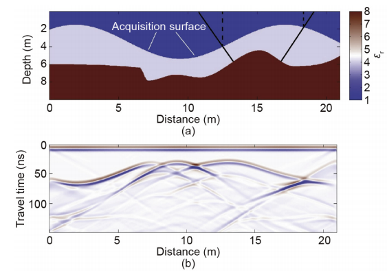
Fig. 1. (a) Schematic of travel paths for a zero offset section, collected along a topographic surface, after correction to a datum: The vertical dashed lines show the travel path, which is implicitly assumed in a standard elevation static correction; the solid lines show the correct travel path; the assumed path is a poor approximation leading to failure of migration from datum after elevation statics corrections (adapted from Ref. [4]). (b) Synthetic GPR data acquired along the acquisition surface shown in (a). εr is relative permittivity.
In this study, we present an RTM post-stack approach for imaging in complex topography based on the exploding reflector concept. The downward wavefield extrapolation is implemented directly from the topographic surface, thereby avoiding the need for elevation statics or datuming. In addition, the algorithm is based on the wave equation solution of Maxwell’s equations, and can account for complex velocity and conductivity distributions. We test the algorithm with synthetic examples and with field data acquired over sand dunes that contain steeply dipping, complex stratigraphy coupled with topographic variations on the same order as the depth-to-target.
《2. The RTM algorithm》
2. The RTM algorithm
RTM is conceptually simple: The recorded wavefield is extrapolated into the subsurface by solving Maxwell’s equations with a negative time step and inserting the radargram as a boundary condition at the surface in reverse time order. In the post-stack case, the imaging condition is met when the clock has counted backward to zero time—that is, when all the recorded energy has been injected back into the model and propagated downward to its point of origin. There are two well-known caveats included in this RTM algorithm. First, the velocity field must be smoothed in order to prevent artificial reflections in the extrapolation process. We use a triangular smoother over two wavelengths at the dominant frequency of the wavelet; this degree of smoothing minimizes spurious reflections at minimal cost to accuracy. The second caveat is that the exploding reflector model properly treats primary reflections only; imaging errors will result if high-amplitude multiples are present in the data. Here, we solve the decoupled, second-order differential form of Maxwell’s equations. In a two-dimensional (2D) system, with the electric field polarized perpendicular to the image plane (transverse electric (TE) mode), these equations are reduced to the damped scalar wave equation:

where E is the electric field, μ is the magnetic permeability, t is time, and x and z are the spatial variables. The variables e and r are the permittivity and electric conductivity. In our algorithm, we assume that the magnetic permeability, l, is equal to the magnetic permeability of free space, μ0. We utilize the low loss approximation in which the loss tangent σ/(ωε)≤1, in which ω is the angular frequency of the wave. In this case, the velocity, v, and attenuation coefficient, α, are as follows:

In the exploding reflector model, the field is approximated with one-way propagation and the model velocity is one-half the value of the true velocity, v' =v/2, where the primed parameter indicates the effective value used in the exploding reflector model. From Eq. (2), it is evident that the exploding reflector solution of Eq. (1) requires the variable substitution ε'=4ε.
To ensure that the primary arrivals undergo the correct amount of attenuation during the one-way propagation, Eq. (3) requires the following:

where z is the depth to the reflector. The right-hand side of Eq. (4) is the attenuation for two-way propagation, while the left-hand side is the attenuation for one-way propagation in the exploding reflector model. After canceling common factors, rearranging, and noting that ε'=4ε, we find the following:

The primed constitutive parameters ε' and σ' are now substituted into Eq. (1) to arrive at our modified wave equation for the exploding reflector model.
We solve the wave equation using a second-order accurate finite difference algorithm, and use perfectly matched layer (PML)-absorbing boundary conditions, as formulated by Zhou et al. [9]; this leads to sets of coupled anisotropic equations to solve in the boundary region. For example, in the z direction, with Zhou et al.’s formulation, the set of differential equations to solve in the boundary region is

where the auxiliary variables D1z and D2z are defined by Eq. (6). The variables σz and αz are the PML absorption parameters.
We implement the algorithm in MATLAB utilizing matrix calculations to gain computational efficiency by taking advantage of multi-core/processor systems. The wavefield extrapolation is computed using Eq. (1), but with a negative time step. The recorded wavefield is input as a boundary condition in reverse time order along the recording or topographic surface. Since the algorithm is computed on a square grid, some error is introduced by the grid discontinuities along the surface. Because these discontinuities are much smaller than a wavelength, the introduced errors are minimal (< λ/10 at the highest frequency in the data). For example, for a 100 MHz Ricker wavelet, the highest frequency contained in the data is approximately 2.5f0, or 250 MHz. With a typical maximum relative permittivity of εr = 9, the grid spacing is 4 cm, compared with the wavelength of 1 m at the dominant 100 MHz frequency. The lack of scattering from the computation grid is a good indicator that the approximation is reasonable.
《3. Synthetic examples》
3. Synthetic examples
《3.1. Synthetic Example 1: Simple velocity structure》
3.1. Synthetic Example 1: Simple velocity structure
We first investigate the effect of large topographic variations with a simple layered velocity structure (Fig. 1(a)). This model has large surface topography variations relative to the depth of investigation—a situation that is often encountered in GPR investigation. The sinusoidal surface topography has a trough-to-peak height of 4 m, and the depth to the irregular reflecting layer varies from 1 to 5 m. There is a single reflecting interface that produces a complicated wavefield in the simulated GPR data (Fig. 1(b)), which shows the triplications characteristic of a reflector with multiple synclines. We consider three processing sequences: ① RTM assuming that the data were acquired on a flat surface followed by elevation statics (Fig. 2(a)); ② elevation statics followed by RTM from datum (Fig. 2(b)); or ③ RTM from topography (Fig. 2(c)). Migrating the data without topography corrections results in large errors; the image is poorly focused and reflections are not correctly located (Fig. 2(a)). The data appear to be over-migrated by between 7 and 10 m, and the anticline between 13 and 18 m appears to be flat. Applying standard elevation corrections followed by migration improves the result, but the image reconstruction still contains large errors (Fig. 2(b)). Note the syncline centered at a distance of 15 m along the profile. It appears to be over-migrated, which could lead to the erroneous conclusion that the velocity model is incorrect (Fig. 2(b)). The image is not correctly focused in the area between 6 and 8 m. This region contains the lowest point of the topography and a steeply dipping short segment on the reflector. Poor focusing results in the appearance of two apparent interfaces in this region. RTM from topography correctly focuses the image and places the reflecting boundary at the correct depth (Fig. 2(c)).
《Fig.2》

Fig. 2. Synthetic data from Fig. 1(b) with three different processing sequences. (a) RTM assuming that the data were acquired on a flat surface followed by elevation statics; (b) elevation statics followed by RTM from datum; (c) RTM from topography. Images in (a) and (b) are poorly focused, while RTM from topography, (c), correctly focuses the image and places the reflecting boundary at the correct depth, as indicated by the solid black line.
《3.2. Synthetic Example 2: Large lateral velocity gradient》
3.2. Synthetic Example 2: Large lateral velocity gradient
A major benefit of RTM is its ability to handle large lateral velocity contrasts. To test both the response of our algorithm to abrupt lateral velocity changes and severe topography relative to the depth of investigation, we constructed the model shown in Fig. 3(a). This model has the same geometry as the model from Example 1, but we have added an abrupt increase in permittivity (decrease in velocity) of the first layer on the left side of the model. The resulting synthetic GPR data are similar to those of Fig. 1(b), but with some notable travel time delays on the left side of the model, where the velocity is lower than in the first model.
Here, we consider only two processing schemes: ① conventional flow with elevation statics followed by RTM, and②RTM from topography. For elevation statics, the higher velocity material was used for the replacement velocity. RTM from datum after elevation statics was carried out with the correct velocity model, yet the image is poorly focused and reflections are not correctly located (Fig. 3(c)). This image is similar to Fig. 2(b). RTM from topography accurately reconstructs the image, producing a sharp image of the reflecting boundary even in the area of large lateral velocity contrast in the overburden (Fig. 3(d)). It is notable that the steeply dipping segment on the reflector (centered at a distance of 7 m) is difficult to image. In this case, the vertical velocity boundary refracts most of the energy reflected from the steep segment away from the surface. The net result is low amplitude in the reconstructed image at this location. It is also notable that the reflection coefficient is smaller on the left side of the model, resulting in a lower amplitude along the interface up to a distance of 10 m.
《Fig.3》

Fig. 3. (a) Synthetic model with sharp lateral contrast in the first layer at a distance of 10 m; (b) synthetic data generated from (a); (c) RTM from datum after elevation statics does a poor job of focusing the image; (d) RTM from topography accurately reconstructs the image even with large lateral velocity gradients, and avoids the need for datuming.
《4. Field test: Coral Pink Sand Dunes, Utah, USA 》
4. Field test: Coral Pink Sand Dunes, Utah, USA
The Coral Pink Sand Dunes (CPSD) are located in southern Utah and are one of the largest dune fields in the Great Basin–Colorado Plateau transition zone. The CPSD rest on Navajo Sandstone, and are bisected by the Sevier normal fault, which also forms the bedrock escarpment along the eastern boundary of the lower dune field (LDF). To test the hypothesis that fault-controlled topography along the underlying bedrock surface controls dune formation and geometry, we carried out a GPR study. Our primary objective was to map the dune–bedrock interface and to image structural features within the bedrock.
We collected over 20 km of profiles along 25 transects with 50 and 100 MHz antennas. Elevation control was maintained using continuous global positioning system (GPS) with differential corrections made in post-processing. The GPS base station was located within 10 km of all transects. The GPS and GPR positions were linked by syncing the GPR acquisition clock to the GPS clock. GPR signal penetration was excellent, and we recorded reflections at depths of greater than 35 m in some locations. This provided excellent images of both the modern dunes and the underlying ancient dune stratigraphy. Outcrops and/or shallow boreholes along some transects provide ground truth for dune–bedrock contacts. While GPR signal quality was excellent, topographic and stratigraphic complexity provided an imaging challenge at the site. Surface topography varied by more than 25 m along some profiles with sustained gradients of greater than 30. This dataset provides a good field example to test our RTM algorithm.
We tested two processing flows: ① RTM after elevation statics, and ② RTM from topography. Processing steps for each flow are listed in Table 1. Critically, we applied migration at a constant permittivity, which we determined by examining the collapse of diffraction hyperbolas after migration at several different permittivity values. Using the same permittivity produced good migration results throughout the survey area. Because the only significant complications are topography and stratigraphy, this dataset is an ideal field example on which to evaluate the RTM from topography approach.
《Table 1 》
Table 1 Processing flows for a comparison of RTM after elevation statics with RTM from topography.

《4.1. Location 1》
4.1. Location 1
Figs. 4 and 5 illustrate a typical profile with some particularly interesting features. In general, we see the modern dune sand lying on top of the bedrock surface, with bedrock composed of ancient lithified dunes. Bedrock is often exposed in the intradune areas. Region 1 is a zone of steeply dipping bedforms within the bedrock stratigraphy. With RTM from datum, the bedforms are poorly focused and appear to be incorrectly placed; for example, the clinoforms to the left appear to cut through an older, deeper surface at a depth of 30–35 m. With RTM from topography, the steeply dipping strata are better focused and appear to be correctly located. Region 2 contains a feature that we have interpreted as a normal fault within the bedrock. With RTM from datum, the fault plane is not well focused, and it is difficult to interpret the relative geometries of the strata and fault. With RTM from topography, the fault plane is well focused and we can see a complicated fracturing geometry. Note that this fault does not appear to offset the erosional contact near the surface and therefore has not likely been active in modern times.
《Fig.4》
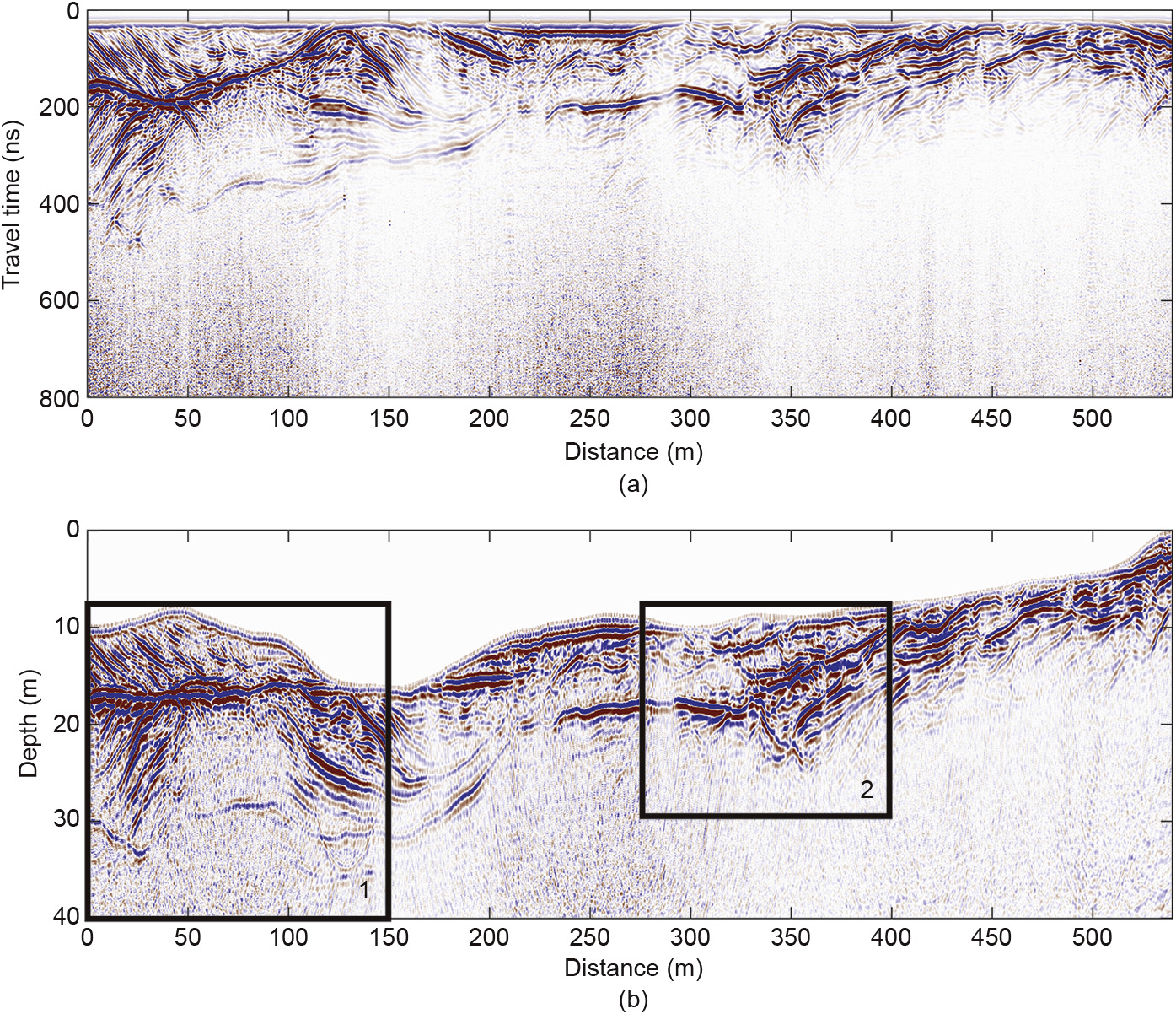
Fig. 4. An example profile from the CPSD survey showing (a) the preprocessed data prior to migration, and (b) the data after RTM from topography.
《Fig.5》

Fig. 5. In Region 1, comparing (a) RTM from datum with (b) RTM from topography, we note the different placement of steep reflections within the bedrock stratigraphy from 20 to 30 mdepth at distances of less than 50 m, and the improved focusing between 100 and 125 m distance when migrated from topography. In Region 2, comparing (c) RTM from datum with (d) RTM from topography, there is an event dipping steeply to the right between 340 and 360 m that we interpret as a normal fault. The fault plane is well focused with RTM from topography, but is difficult to interpret when migrated from datum.
《4.2. Location 2》
4.2. Location 2
Fig. 6 illustrates some of the complexities we observed in the modern dune structures. The profile crosses two 7 m high dunes, and is oriented perpendicular to the dune axis. The dunes are resting directly on the bedrock surface with only a thin covering of sand in the intradune areas. Consider the steep, leftward-dipping, leeward face of the dune on the right of the profile. Where the steep face of the dune intersects the approximately horizontal intradune surface, RTM from datum severely misplaces the bedrock surface, making it appear that bedrock is outcropping just above the dune base; however, bedrock was definitely not outcropping. RTM from topography correctly places the bedrock surface, and we find that the bedrock dips just beneath a thin covering of sand.
《Fig.6》

Fig. 6. (a) Preprocessed data from a line in the central part of the dune field collected with a 100 MHz antenna; (b) data after RTM from topography, where the internal stratigraphy of the dunes and the bedrock interface are clear; (c) right-hand dune shown after RTM from datum; (d) the same dune after RTM from topography. At the transition from the base of the dune to the dune face, the bedrock surface is clearly misplaced when migrated from datum. In addition, steeply dipping internal reflectors are better focused after RTM from topography.
《5. Discussion and conclusions 》
5. Discussion and conclusions
When imaging complex stratigraphy beneath rugged topography, the kinematics of the recorded wavefield deviate significantly from the assumption of vertical near-surface propagation that is implicit in standard elevation static corrections. RTM from datum after such corrections significantly distorts the image, leading to poor focusing and incorrect positioning of reflections. RTM from topography correctly treats the wavefield kinematics and produces an accurate image, even in the presence of large lateral velocity gradients. Precise horizontal and vertical surveying is critical to producing an accurate image.
The exploding reflector model we implement here utilizes the second-order decoupled form of Maxwell’s equations. Since the magnetic field is not computed directly, as in the Yee algorithm, this approach has the computational advantage of computing and storing only the electric field. The exploding reflector model used in the imaging algorithm discussed in this study properly accounts for the primary arrival only; significant imaging errors will occur if large multiples are contained in the data. Finally, smoothing of the velocity model is required for the RTM procedure in order to avoid artificial reflections during the wavefield extrapolation. With these caveats, the case studies presented here illustrate that post-stack RTM is a valuable tool when producing accurate images in complex and rugged environments is critical. An accurate migration result depends on an accurate velocity model. When the velocity structure is more complicated than that which was encountered at the CPSD, a more rigorous approach to velocity estimation will be required, such as multi-channel, multi-offset acquisition with reflection tomography. With multioffset data, it is possible to utilize pre-stack RTM with the full two-way wave equation, thereby avoiding the one-way propagation approximations that are required in the exploding reflector model. Additional field examples of both pre- and post-stack RTM GPR imaging will improve our understanding of the benefits and limitations of this computationally intensive imaging technique.
《Acknowledgements 》
Acknowledgements
The Herbette Foundation at the University of Lausanne provided support for the development of the RTM algorithm.
《Compliance with ethics guidelines 》
Compliance with ethics guidelines
John H. Bradford, Janna Privette, David Wilkins, and Richard Ford declare that they have no conflict of interest or financial conflicts to disclose


 京公网安备 11010502051620号


