《1. Introduction 》

1. Introduction

Dental cavity preparation is a basic clinical operation skill in oral medicine. The cavity, which is used to contain filler material in order to restore the shape and function of the tooth, is formed by removing caries lesion with dental surgery. Rigorous criteria for the cavity in terms of depth, length, width, and angle make its assessment an important work in clinical teaching. Digital assessment that uses computer-assisted three-dimensional (3D) reconstruction has now become an important means for dental teaching; however, the digital assessment systems that are mainly used are expensive and still need to be improved in terms of blind area and precision [1,2]. 3D laser scanning has the advantages of high precision, fast speed, and easy implementation [3–6]. This method projects the laser onto the object and collects images of the object with the laser stripe, thus actively forming triangle similarity relationships between the images and objects. Calibration is critical for laser scanning, as it determines the validity and precision of the measurement results.

There are two main problems in calibration. The first is the question of how to collect a substantial number of accurate calibrating points using appropriate methods. The wire-drawing method [7] and dentiform bar method [8] that were proposed early depend on expensive external equipment and gain few calibrating points. Although Huynh et al.[9] achieved high-precision calibrating points based on the invariance of the cross-ratio, these calibrating points are sometimes insufficient. At present, a planar target is widely used to collect the calibrating points due to its simple fabrication and flexible operation [10–12]. For a rotation scan, the rotation axis must also be calibrated [13–15]. Most of the abovementioned methods involve complicated artificial operations. Convenient calibration is becoming important, because recalibration must be done frequently in order to eliminate errors caused by movements or environmental changes.

The second problem is how to calculate the parameters using an appropriate algorithm. Calibration algorithms can be divided into two types: the mathematical method and the machine-learning method. The mathematical method establishes mathematical formulas according to the principle of 3D laser scanning. Due to imaging restorations, structure errors, and other uncertainties, complete and precise mathematical formulas usually turn out to be very complex. The machine-learning method builds transformation relations between image coordinates and spatial coordinates directly using artificial neural networks (ANNs) and genetic algorithms [16,17]. As a black box algorithm, the machine-learning method does not require camera calibration and mathematical formulas; however, it has disadvantages such as low convergence and poor generalization. This paper presents a dual-platform scanner for dental reconstruction and assessment, and proposes a method of hybrid calibration for laser scanning to improve the convenience and precision.

《2. Methodologies 》

2. Methodologies

《2.1. Laser scanning 》

2.1. Laser scanning

In 3D laser scanning, when the line of the laser is projected onto the object being measured, an image of the part of the object with the light stripe is acquired by the camera, as shown in Fig. 1. If P is a point on the object being measured, its image P' appears to be on the light stripe in the image plane when it is scanned by the laser. The world coordinates frame o_wx_wy_wz_w describes the 3D information of the object. The camera coordinates frame o_cx_cy_cz_c and the image coordinates frame o₀xy are established with an origin of o_c and o₀, where o_c is the optical center and o₀ is the intersection of the optical axis and image plane. The distance between o_c and o₀ is f, which is also called the focal length. The pixel array on a complementary metal-oxide semiconductor (CMOS) camera is expressed by ouv. As the position of P' in the ouv can be found through image processing, the principle is to derive the transformation from ouv to o_wx_wy_wz_w.

《Fig.1》

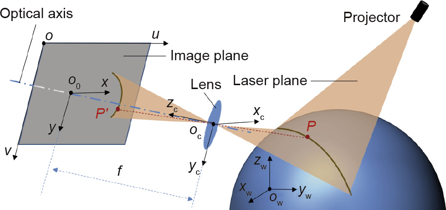
Fig. 1. Principle of 3D laser scanning

If the subscript of o₀ in the pixels array is (u₀, v₀), then the transformation from ouv to o₀xy is

where s_x and s_y, as given by the camera manufacturer, are the physical dimensions of a pixel on the CMOS camera in the corresponding direction.

In the ideal pinhole imaging model of the camera, the proportional relationship between P (x_c, y_c, z_c) and P'(x, y) is

The transformation from o₀xy to o_cx_cy_cz_c is based on this proportional relationship, which is usually expressed in the form of a homogeneous matrix, as follows:

Meanwhile, a rigid body transformation occurs between o_wx_wy_wz_w and o_cx_cy_cz_c in 3D space. Supposing that R is a 3×3 rotation matrix and T is a translation vector, the transformation is

Thus, we can derive the transformation from ouv to o_wx_wy_wz_w from Eqs. (1), (3), and (4).

Eq. (5) is the camera model, where M₁ is the intrinsic parameter matrix and M₂ is the extrinsic parameter matrix. The model can also be written as a projection matrix M, as shown in Eq. (6).

In 3D laser scanning, the world coordinates axis x_w is usually parallel to the scanning direction, so x_w can be acquired directly by the scanner. The other 3D information, (y_w, z_w) , is worked out by eliminating z_c in Eq. (6):

Eq. (7) is the basic model of 3D laser scanning. This is an ideal model under ideal conditions. However, a variety of nonlinear distortions occur in practical application. The main distortions that affect the imaging results are radial distortion and tangential distortion [18]. Radial distortion and tangential distortion come from the shape of the lens and the assembly of the camera, respectively. Their distortion models are

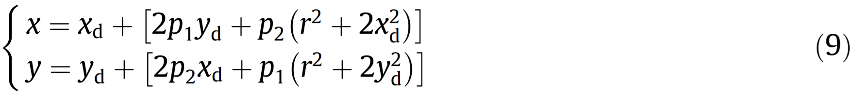
where x_d and y_d are real imaging positions; x and y are ideal imaging positions; r² = x²_d + y²_d; k₁, k₂, and k₃ are radial distortion coefficients; p₁ and p₂ are tangential distortion coefficients. In this case, f, u₀, v₀, R, T, k₁, k₂, k₃, p₁, and p₂ need to be determined through calibration before the scanner begins the measurement.

《2.2. Calibration methods》

2.2. Calibration methods

As stated above, calibration establishes the transformation relationships between the pixel array (u, v) and the world coordinates (y_w, z_w). In general, there are two kinds of method: the mathematical method and the machine-learning method.

The mathematical method establishes mathematical formulas based on the calibration principle first, and then works out the unknown parameters of these formulas through nonlinear optimization. The Tsai’s two-step method [19] and the Zhang’s method [20] are the most widely used forms of the mathematical method. The Tsai’s two-step method uses a 3D calibration target, while the Zhang’s method uses a planar calibration target. In the Zhang’s method, several planes in different positions are used to calculate the parameters, because points on each plane can be used to set up two equations. Zhang’s calculated the initial values of the parameters under the assumption of no distortion, and then worked out distortion coefficients with these initial values by the least squares method. Precision is optimized by maximum likelihood estimation.

In the Tsai’s two-step method, since only quadratic radial distortion is considered, the radial arrangement constraint is applied:

Because (u₀, v₀) can be determined through the optical method, (x_d, y_d) are known data. The intermediate parameters, r₁/t_y, r₂/t_y, r₃/t_y, t_x/t_y, r₄/t_y, r₅/t_y, and r₆/t_y, can be worked out from Eq. (10), if there are more than seven calibrating points. First, the extrinsic parameters, R, t_x, and t_y, are calculated based on the orthogonality of the rotation matrix. The other parameters, f, k₁, and t_z, are approached based on the camera and distortion model by nonlinear optimization.

The machine-learning method establishes the transformation relationship between the input (u, v) and output (y_w, z_w) directly by training sample data. In essence, this is a black box method that requires no intrinsic or extrinsic parameters. ANNs are typical machine-learning algorithms. For example, the back-propagation network (BPN, which is a kind of ANN) has been shown to be an effective method for building nonlinear mapping relationships with high versatility and precision [21,22]. With the steepest descent method, the BPN can adjust its weights and thresholds to learn the mapping relationship according to the backpropagation errors. As shown in Fig. 2, its structure consists of an input layer, hide layer, and output layer. Each layer has several nodes that are similar to biological nerve cells.

《Fig.2》

Fig. 2. Structure of a three-layer BPN.

The learning process of the BPN has two directions. The forward propagation of data realizes an estimated mapping relationship from n dimensions to m dimensions, while the back propagation of errors helps to revise this mapping relationship. In forward propagation, the input data flow to the hide layer and then to the output layer. For a nude h_k in the hide layer, the value is determined by the threshold a_k, the related input data x_i, and the corresponding weights v_ki:

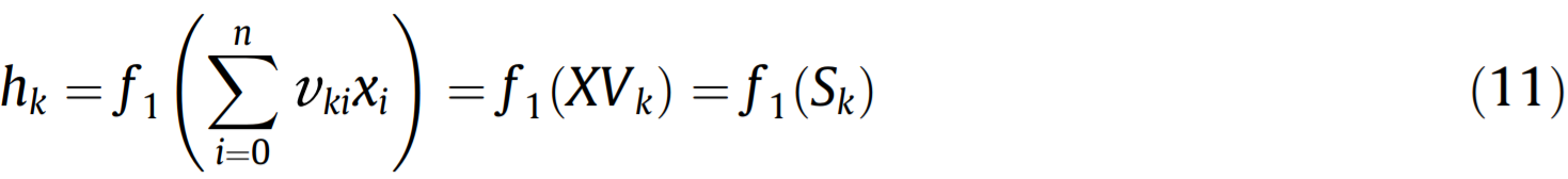
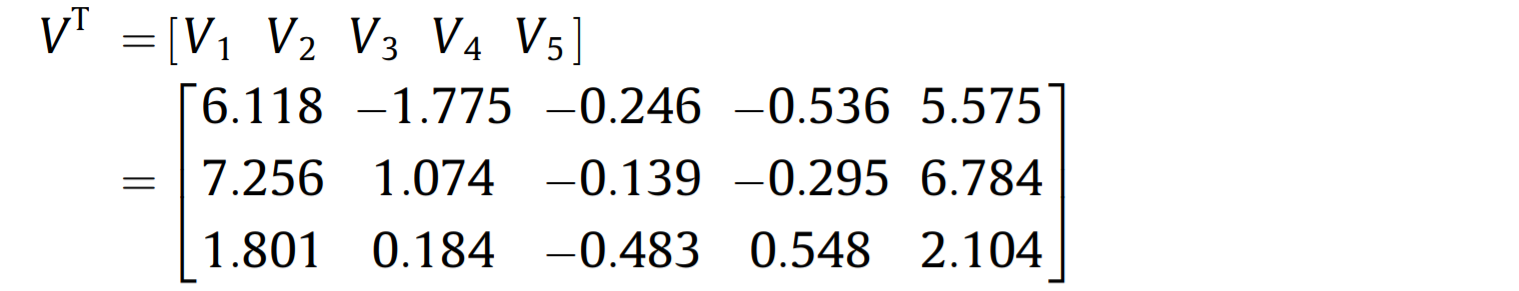
where V_k = [a_k  v_k1  v_ki  ... v_kn]^T , X = [ 1  x₁  x_i  ...  x_n ], f₁ is the activation function, and S_k is the node’s net input. Similarly, for a nude y_j in the output layer, the value is determined by the threshold b_j, the related h_k, and the corresponding weights w_jk.

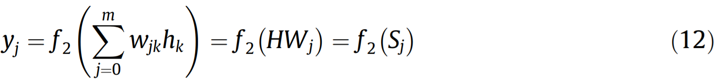
where W_j = [b_j  w_j1  w_jk ... w_jq]^T , H = [1  h₁  h_i ... h_q ], f₂ is the activation function, and S_j is the node net input. In back propagation, the errors between the desired output and the actual output are used to adjust the weights and thresholds in order to minimize the global error function. If the size of the learning samples is P, then the global error function is:

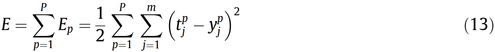
where E_p is the error of the pth sample and t^p_j is the desired output. Changes in the weights and thresholds are calculated based on the partial differential of E_p with a learning rate of η, which in the output layer and the hide layer is:

Eq. (14) can be deduced into a specific form through the chain rule:

The network structure gives the BPN a strong nonlinear mapping ability. To apply the BPN, (u, v) and (y_w, z_w) are seen as input and output data. The calibration can be completed by a learning process based on Eqs. (11), (12), and (15).

The mathematical method is specific and robust, but it is diffi- cult to work out the mass of the parameters. The mathematical formulas usually only concern the main distortions to be kept simple, which makes the formulas unable to handle other nonlinear factors and uncertainties. The machine-learning method can deal with all the imaging restorations, structure errors, and other uncertainties. Thus, it seems to be quite appropriate for the calibration of laser scanning. However, the expected results cannot be achieved in practice. In addition, this method is apt to plunge into the local minimum, in what is known as over fitting or poor generalization. Poor generalization means that the network performs rather worse with testing samples than with training samples. In this case, only the calibrating points can be measured. In general, the distortions and errors are two orders of magnitude smaller than the ideal values determined by the basic model. Both the mathematical and machine-learning methods process the data directly, which causes the distortions and errors to be concealed by the ideal values. This is an important influencing factor on precision that has been ignored. It can be revealed by normalization, which is a common step in data processing:

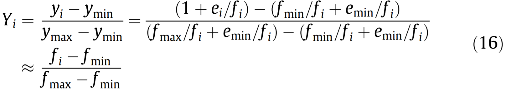
where y is the sample data, which consists of the ideal value f and the residual part e that contains distortions and errors. In Eq. (16), both sides are divided by f_i. Since e/f is close to zero, the final normalization value is close to that of the ideal model.

《3. The dual-platform laser scanner》

3. The dual-platform laser scanner

In this paper, a dual-platform laser scanner based on the laserscanning principle is designed for the 3D reconstruction of dental pieces. In dental cavity preparation, the cavity may be on the front or lateral of a tooth. Dental pieces with a cavity on the lateral can only be scanned by means of a rotation platform, whereas those with a cavity on the front are suitable for a translation platform. The dual-platform structure makes it possible to scan all types of dental model with the 3D laser scanner system. As shown in Fig. 3, the scanner consists of two cameras, a laser transmitter, and two platforms. The rotation platform is fixed to the translation platform, so it is possible to switch over the working platform through the translation platform. When in rotation scan mode, the rotation center O_r is moved in the laser plane according to the mark on the rotation platform. The rotation platform maintains a dip, β, with the horizontal x_wo_wy_w plane in order to ensure that the object can be scanned entirely. Two cameras are used in the system to collect images from different sides; this effectively eliminates blind areas and ensures the integrity of the point cloud.

《Fig.3》

Fig. 3. Design of the dual-platform laser scanner.

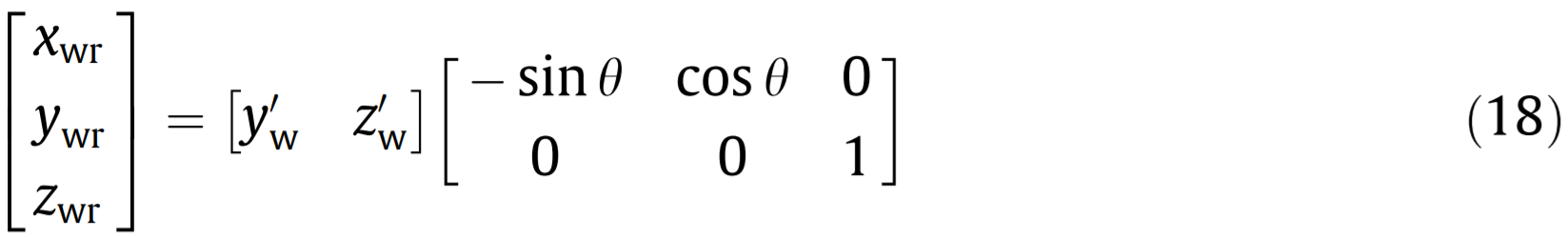
In the translation scan, the direction of the x_w axis is set parallel to the movement of the translation platform. This direction is perpendicular to that of the laser plane, which is also the plane of y_wo_wz_w. When the system operates, the x_w coordinates are obtained from the control module of the translation platform. Simultaneously, (y_w, z_w) are calculated based on the calibration results. In the rotation scan, the scanner obtains a set of twodimensional (2D) physical coordinates (y_w, z_w) each time the rotation platform revolves. These physical coordinates must be transformed and assembled into the 3D point cloud (x_wr, y_wr, z_wr). There are two steps in this process. First, eliminate the tilt of the rotation platform with the dip β and the rotation center O_r (y_r, z_r) , as shown in Eq. (17). Second, assemble the physical coordinates together one by one according to the rotated angle θ, as shown in Eq. (18). The rotated angle θ can be obtained from the control module of the rotation platform, whereas β and O_r (y_r, z_r) need additional calibration.

A dual-platform laser scanner was constructed, as shown in Fig. 4(a). Each camera had a resolution of 1280 ×1024 and an effective view field of 20 mm ×18 mm. The physical dimensions, s_x and s_y, of a pixel were 5.2 μm× 5.2 μm. The calibration target for the translation scan was a stepped gauge with five smooth treads, as shown in Fig. 4(b). Each step had a height of 2 mm, and a length and width of 20 mm×5 mm. The calibration target for the rotation scan was a pattern, as shown in Fig. 4(c). A white circle with a diameter of 10 mm was positioned in the middle.

《Fig.4》

Fig. 4. Experimental facilities for the dual-platform laser scanner. (a) The dualplatform laser scanner; (b) the translation platform and gauge; (c) the rotation platform and pattern.

《4. Hybrid calibrations 》

4. Hybrid calibrations

For the dual-platform scanner, calibration involves finding the coordinate transformation from image coordinates to world coordinates in the translation scan first; next, the dip β and O_r(y_r, z_r) is found in the rotation scan. We use an integrative method to collect the calibrating points. The integrative method can conveniently collect a substantial number of calibrating points and can perform an integrative calibration for both the translation and rotation scans. Furthermore, we propose a hybrid algorithm to establish an effective model. This hybrid algorithm can achieve higher precision by combining the mathematical and machinelearning methods.

《4.1. Integrative method 》

4.1. Integrative method

In the calibration of the translation scan, the stepped gauge is placed on the translation platform. When the stepped gauge moves with the translation platform, the laser projects onto different treads. The images of the treads obtained with the laser can be processed to extract a substantial number of calibrating points. The centers of the light stripe on the image are extracted as image coordinates through the Gaussian fitting method [23], while the world coordinates are gained from the physical dimension. In addition, the transformation of coordinates from image coordinates to world coordinates can be performed through the hybrid algorithm. In the calibration of the rotation scan, the pattern is pasted on the rotation platform. The coordinates of a line on the rotation platform are gained through transformation. The dip β is calculated by the slope of this line. Because the center of rotation is on the laser plane, O_r can be determined through two images that are snapped before and after rotating by 180°. As shown in Fig. 5, P₁ refers to the endpoints of the light stripe on the pattern. The corresponding points after rotating by 180 are referred to as P'₁. P₁ and P'₁ are symmetrical to O_r, which can be used to calibrate O_r ( y_r, z_r) . In general, it is necessary to collect data and perform the calibration several times; the average result is the final result. Next, P₂ and P'₂ are used to calculate the error in the calibration results after these results are obtained.

《Fig.5》

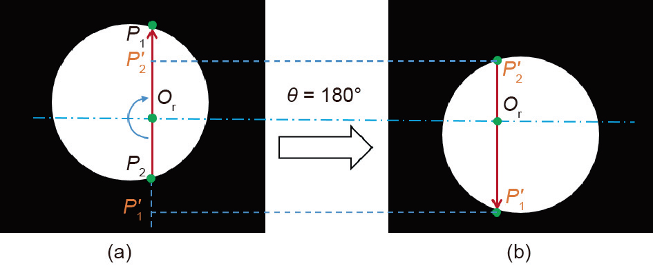
Fig. 5. The symmetrical property of the rotation scan. (a) Initial position; (b) rotated 180°.

《4.2. Hybrid algorithm》

4.2. Hybrid algorithm

Based on the discussion on calibrating algorithms, we propose a hybrid algorithm that combines the mathematical method and the machine-learning method. In this hybrid algorithm, the mapping relationship is divided into two parts: the main part and the compensation part. The main part is determined by the basic model of laser scanning, while the compensation part contains all the distortions and errors, as shown in Fig. 6. The final mapping relationship is made up of the basic model and the network. To establish the hybrid model, the mathematical method is used first in order to work out the basic model. Next, taking the residual between the main part and the real value as the output, the machine-learning method is used to establish the network.

《Fig.6》

Fig. 6. The hybrid algorithm

The basic model is provided in Eq. (7); this can be replaced by the following:

Its matrix form is

where

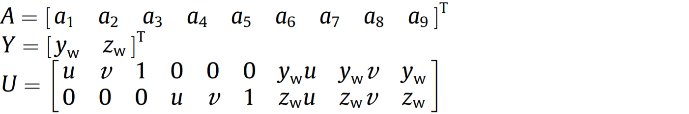
In calibration, since there are far more calibrating points than unknowns, a₁ – a₉ can be worked out through the least squares method:

The BPN is used as compensation in order to learn the mapping relationship of the distortion and errors. The input data are the pixels array (u, v), while the output data are the residual E(e_x, e_y)  between the main part and the real value Y_real.

The network has three layers, with two nodes in the input layer and two nodes in the output layer. The hybrid algorithm is superior to the mathematical and machine-learning methods, as it combines the advantages of both methods while overcoming their shortcomings. When compared with a pure mathematical method, the hybrid model is more complete than the mathematical formulas, because all the distortions and other errors can be compensated for by the network. When compared with a pure machine-learning method, the hybrid model is more specific and robust, because it is no longer a black box network. The basic model ensures the main part of the mapping relationship and improves the generalization ability, which can limit the generalization error to the residual level of E(e_x, e_y). The hybrid algorithm has higher precision in calibration, because it can diminish the influence of ideal values on the distortions and errors. It divides the mapping relationship into two parts at the beginning, thus avoiding the concealing problem shown in Eq. (16).

《5. 3D reconstruction》

5. 3D reconstruction

The result of laser scanning is point-cloud data, which needs to be simplified and reconstructed in order to restore the 3D shape of the object.

《5.1. Point-cloud reduction 》

5.1. Point-cloud reduction

The initial point cloud contains many redundant points; this increases the amount of computation and reduces the efficiency of reconstruction. Therefore, it is necessary to simplify the point cloud before triangulation. We propose a point-cloud simplification method in order to process point-cloud data according to the morphological characteristics of the point cloud. This method has higher processing efficiency and a better streamlining effect.

For the point cloud that is obtained by translational scanning, the density of the point-cloud distribution is larger in the direction of the light bar and smaller in the scanning direction; therefore, there are many redundant points in the direction of the light bar, as shown in Fig. 7. In order to preserve the feature information of the point clouds, it is necessary to calculate the distance between adjacent points on the stripe. If the distance is greater than the threshold, these points contain more feature information and should be preserved. The rest of the points are sampled randomly according to the density of the point clouds in the scanning direction.

《Fig.7》

Fig. 7. The translational scanning point cloud.

For the point cloud that is obtained by rotational scanning, the point-cloud data are radially distributed around the rotational center. The closer it is to the rotational center, the higher the pointcloud density is and the more redundant points there are, as shown in Fig. 8. Therefore, the point-cloud data can be divided into n concentric circle regions around the center of rotation. The radii of the concentric circle are r, , , ...,  and the area of each concentric circle is equal. According to the distribution characteristics of point clouds, the number of points in each ring is proportional to the width of the ring. If the ratio is k, the point-cloud density of the first ring is

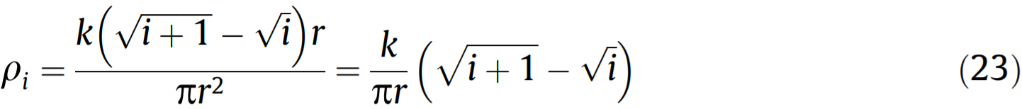
According to the density of the point clouds in each concentric ring, we set a simplified threshold in order to simplify the point cloud. Finally, a complete point cloud with uniform distribution and more feature information is obtained.

《Fig.8》

Fig. 8. The rotational scanning point cloud.

《5.2. Delaunay triangulation》

5.2. Delaunay triangulation

A triangular mesh occupies less storage space and represents better surface fineness; thus, it has become the main means of realizing 3D display in a computer. In general, there are two ways to triangulate 3D point-cloud data: first, directly triangulating 3D points; and second, projecting 3D points onto the 2D plane, using 2D plane triangulation to create meshes. The former way has a large computation and the algorithm is not stable. 2D planar triangulation has a good theoretical basis and good mathematical characteristics, but it is only suitable for surfaces that are projected in a certain direction without overlapping.

According to the principle of translational scanning, as shown in Fig. 3, the point-cloud data obtained by the translational scanning of line-structured light can actually be regarded as the projection of the object in the x_wo_wy_w plane. Therefore, the translational scanning point cloud represents a surface projected onto the x_wo_wy_w without overlap, which can be directly projected through two dimensions transformation, using the Watson’s algorithm for triangulation [24]. The Delaunay triangulation process using the Watson’s algorithm is as follows: ① build a super triangle DE that contains all the points; ② insert a new point from the point set and connect it to the three vertices of the triangle ∆E in order to form the initial mesh; ③ insert a new point and find the "influence triangle,” which is the triangle containing the point; ④ delete the common edge of the "influence triangle” and connect the new point to the related vertices in order to form a new mesh; ⑤ repeat ③ and ④ until all of the points in the point set are processed.

Because of the characteristics of the revolving body, the rotational scanning point cloud has overlapping problems in any direction. Therefore, point clouds cannot be directly triangulated through 2D projections. Considering the acquisition process of the rotational point cloud, the point-cloud data are obtained by line-structured light projection before tilting and splicing. Therefore, the rotating point cloud can be tilted and expanded according to the scanning position by coordinate transformation. The expanded point cloud has the shape of a linear-structured light projection and can be triangulated by 2D projection. It is necessary to combine the triangular mesh together after the point cloud is triangulated in order to finally obtain the complete subdivision of the rotating point cloud.

The triangulation of the rotational scanning point cloud can be summarized as follows: ① divide the rotational point cloud into four regions, A, B, C, and D, and ensure that A, B, C, and D have overlapping boundary points, as shown in Fig. 9; ② transform the coordinates of each region with the center of rotation and expand the point cloud into the shape before tilting and splicing; ③ at this time, every area forms a surface that does not overlap the x_wo_wy_w plane itself; ④ triangulate the point cloud of each region; ⑤ after the 2D projective triangulation of each region is complete, put the triangular mesh together to form the complete mesh of the original point cloud, according to the overlapping boundary points of the four regions.

《Fig.9》

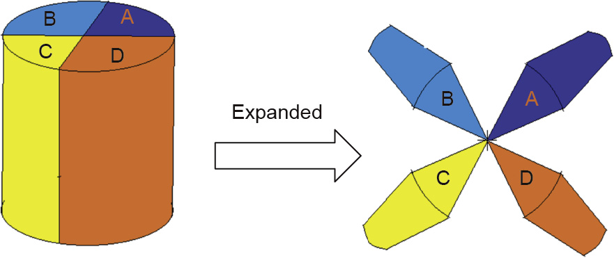
Fig. 9. Dividing and expanding the original point cloud.

《6. Experiments and results 》

6. Experiments and results

Experiments using the Tsai’s two-step method, the BPN method, and the hybrid method were conducted in order to demonstrate the validity of the hybrid calibration. Measurement and reconstruction results after calibration were obtained.

《6.1. Calibration 》

6.1. Calibration

6.1.1. Data collection

The points were collected by placing the stepped gauge on the translation platform with its first tread under the laser. As the world coordinates frame was set based on the physical dimensions of the gauge, the remaining steps were performed automatically through programmatic control. This section introduces the experiment based on the left camera. The images of the treads that were collected in the experiment are shown in Fig. 10. A total of 5038 valid samples were collected after image processing; these were used for the calibration of the translation scan by establishing the coordinate transformation. A pair of symmetrical pattern images that were collected in the experiment is shown in Fig. 11. Since the interval angle was 15°, a total of 12 pairs of symmetrical images were used for the calibration of the rotation scan.

《Fig.10》

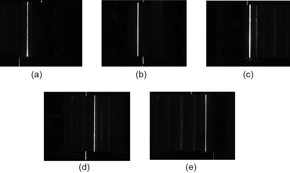
Fig. 10. Image acquisition of the target. (a) First, (b) second, (c) third, (d) forth, and (e) fifth tread.

《Fig.11》

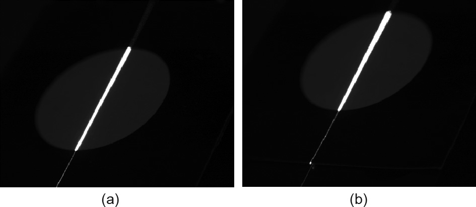
Fig. 11. Image acquisition of the pattern. (a) θ = 0°; (b) θ = 180°.

6.1.2. Calibration results

Based on the hybrid algorithm, the basic model was worked out using Eq. (21). The compensation network was a three-layer BPN with five hide nodes, which was trained 100 times with a terminal of 10^-4 . β and O_r can be calculated in each pair, with the average taken as the final value. The parameters of the basic model and the network are provided below: A = [-0.027  1.038  -19.580  -1.997  -0.003  1262.001  -0.007  0  44.987]

β = 44.320°

O_r(5.451, 4.397)

Calibrations were also conducted with the Tsai’s two-step method and the pure BPN method as contrasting experiments. The calibration results of the Tsai’s method are given below:

[f  k₁  u_o  v_o] = [41.397  0.0001  637  509]

β = 44.761°

O_r(5.141, 4.580)

In the pure BPN method, the network was also three layers with five hide nodes. After being trained 100 times with a terminal of 10^-4 , its parameters were as follows:

β = 43.832°

O_r(5.159, 4.032)

6.1.3. Discussion

The stepped gauge was scanned using different methods, and five equally spaced points were picked up on each tread. In this case, the points on each tread were uniformly distributed along the x axis of the image plane, while the treads were uniformly ordered along the y axis. A reference plane that was 2 mm below the first tread was also scanned; it imaged on the edge of the pixels array and was used to test the generalization ability. The distribution and statistics of the errors are shown in Fig. 12 and Table 1. The performances of the networks in the pure BPN method and the hybrid method are shown in Fig. 13. For the rotation scan, the endpoints on the pattern were picked out in order to calculate the errors in the rotation scan, as shown in Fig. 14 and Table 1.

《Fig.12》

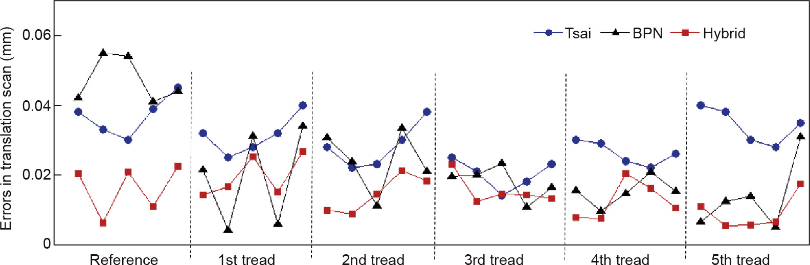
Fig. 12. Errors in the translation scan.

《Fig.13》

Fig. 13. Performance of (a) pure BPN and (b) hybrid BPN. MSE: mean squared error.

《Fig.14》

Fig. 14. Errors in the rotation scan.

《Table 1 》

Table 1 Error statistics.

As shown in Fig. 12, the Tsai’s method has regular, steady errors. For the whole gauge, the treads close to the middle had smaller errors than those close to the edge. For each tread, the points close to the middle had smaller errors than those close to the edge. Errors in the reference plane were the worst, but still followed this regularity. This distribution is very similar to the distortions, which explains where the errors mainly come from. The root mean square (RMS) errors in the translation scan and rotation scan were 0.030 and 0.056 mm, respectively. The BPN method seems to perform better than the Tsai’s method on the treads, even with the irregularly distributed errors. However, on the reference plane, the errors turned out to be much bigger suddenly, which was caused by the poor generalization ability of this method. As a result, the overall RMS of the BPN in the translation scan and rotation scan reached 0.027 and 0.060 mm, respectively. The hybrid method achieved the best performance in this experiment. It has the smallest errors when compared with the Tsai’s method and the BPN method. The RMS of the errors was 0.016 and 0.031 mm. The basic model ensures steady errors, even on the reference plane. The separation of ideal values and errors also improves the performance of the network. As shown in Fig. 13, for the network in the hybrid method, the mean squared error (MSE) drops 0.0014612 at epoch 19, while that in the pure BPN method is 0.0014651 at epoch 932. The convergence rate of the MSE is much faster in the hybrid method than in the pure BPN method. The dental mold measurement error is required to be less than 0.2 mm, so our measurement method satisfies the accuracy requirements.

《6.2. Measurement 》

6.2. Measurement

Typical dental pieces measured by means of a translation scan and rotation scan, respectively, are shown in Figs. 15 and 16. The measurement results and reconstruction process are shown in Figs. 17 and 18. Fig. 17(a) is the primary point cloud with a total of 37 983 points, while Fig. 17(b) is the point cloud after de-noising and reduction, with a total number of points that has decreased to 6218. Fig. 17(c) shows the result of the Delaunay triangulation. The final 3D reconstruction is shown in Fig. 17(d). Fig. 18(a) is the primary point cloud, which contains many redundant points. After reduction, the number of points is reduced from 87 458 to 6267, as shown in Fig. 18(b). The Delaunay triangulation and the final 3D reconstruction are shown in Fig. 18(c) and (d). The results meet the requirements for dental application.

《Fig.15》

Fig. 15. A typical dental piece for a translation scan.

《Fig.16》

Fig. 16. A typical dental piece for a rotation scan.

《Fig.17》

Fig. 17. Reconstruction of translation scan. (a) The primary point cloud; (b) point cloud after de-noising and reduction; (c) the result of the Delaunay triangulation; (d) the final 3D reconstruction.

《Fig.18》

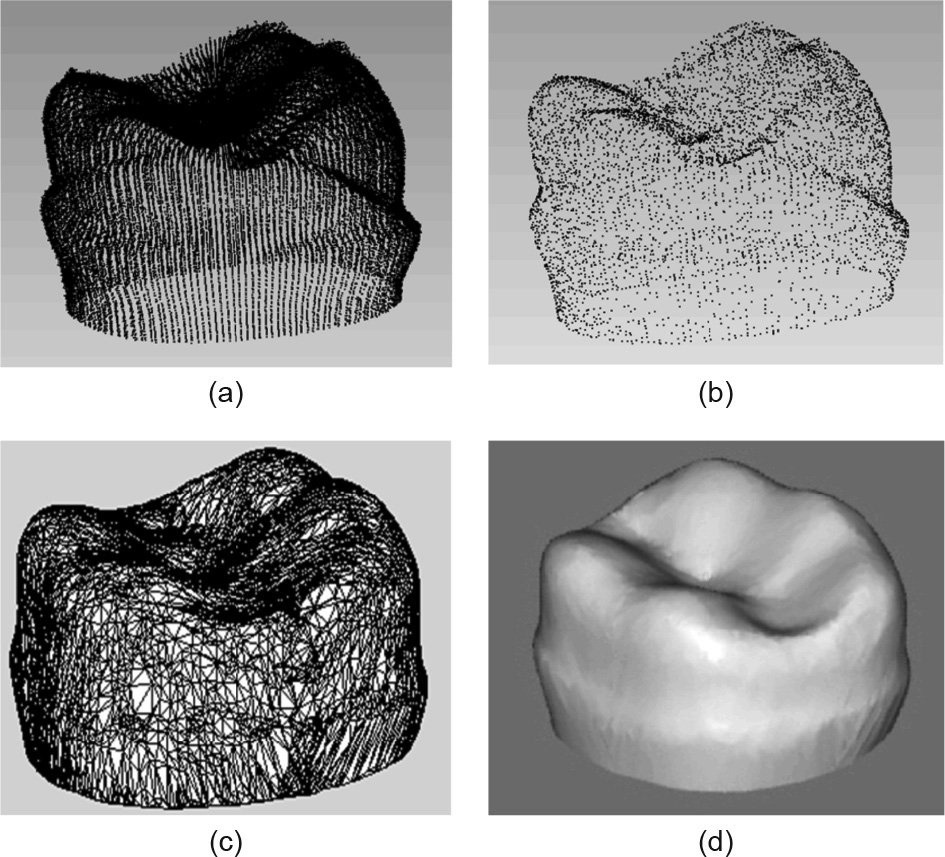
Fig. 18. Reconstruction of rotation scan. (a) The primary point cloud; (b) point cloud after de-noising and reduction; (c) the result of the Delaunay triangulation; (d) the final 3D reconstruction.

《7. Conclusions 》

7. Conclusions

This paper developed a dual-platform laser scanner and proposed a hybrid calibration method for 3D laser scanning for the 3D reconstruction of dental pieces. The dual-platform scanner has a low cost and is suitable for different dental pieces. The hybrid calibration, which includes an integrative method for data collection and a hybrid algorithm for data processing, achieves convenient operation and high precision. The integrative method is able to collect a substantial number of accurate calibrating points by means of a stepped gauge and a pattern with little human intervention. The hybrid algorithm synthesizes the advantages of the mathematical and machine-learning methods through the combination of a basic model and a compensation network. The calibration experiments verified the excellent performance of the hybrid calibration, which had strong stability and a small degree of errors. Two typical dental pieces were measured in order to demonstrate the validity of the measurement performed using the dual-platform scanner. This method provides an effective way for the 3D reconstruction of dental pieces in clinical teaching.

The dual-platform laser scanner can also be applied to the 3D measurement of objects with irregular surfaces, such as the reconstruction of sculptures and artifacts, the measurement of complex industrial parts, and rapid reverse engineering combined with 3D printing. However, the dual-platform laser scanner is bulky and not portable. The scanning process is thus limited by the mechanical platform.

《Acknowledgements 》

Acknowledgements

The authors are grateful for support from the National Science Fund for Excellent Young Scholars (51722509), the National Natural Science Foundation of China (51575440), the National Key R&D Program of China (2017YFB1104700), and the Shaanxi Science and Technology Project (2016GY-011).

《Compliance with ethics guidelines》

Compliance with ethics guidelines

Shuming Yang, Xinyu Shi, Guofeng Zhang, and Changshuo Lv declare that they have no conflict of interest or financial conflicts to disclose.