

《1. Introduction》
1. Introduction
Additive manufacturing (AM), as opposed to traditional subtractive manufacturing technologies, is a promising digital approach for the modern industrial paradigm that has gained widespread interest all over the world [1–4]. By fabricating objects layer by layer from three-dimensional (3D) computer-aided design (CAD) models, AM provides several benefits: ① It creates products with complex shapes, such as topologically optimized structures, which are difficult to manufacture with traditional casting or forging processes; ② it can be used to generate novel characteristics of materials, such as dislocation networks [5], which are very attractive to academic researchers; and ③ it reduces material waste and thus saves on cost for industry. However, AM parts also present dozens of unique defects that differ from those that appear in their cast and wrought counterparts; these include porosity due to a lack of fusion and gas entrapment, heavily anisotropic microstructure in both the perpendicular and parallel directions relative to the printing direction, and distortion due to large residual stress introduced by a high cooling rate and steep temperature gradient [6]. It is thus essential to better understand the complex relationship between a powder’s metallurgical parameters, the printing process, and the microstructure and mechanical properties of AM parts. The AM process always involves many essential parameters that can determine the final products’ performance. For example, in selective laser melting (SLM), the processing parameters—which include laser power, scan speed, hatch spacing, and layer thickness—all significantly affect the quality of the produced parts. Unfortunately, the relationship between these parameters and the output quality is too complicated to fully understand, as SLM is a multi-physics and multiscale process that includes powderlaser interaction at the microscale, melt pool dynamics and columnar grain growth at the mesoscale, and thermal–mechanical coupling at the macroscale. Researchers have tried to develop various physical models in order to classify this relationship in a clearer and more accurate way. Acharya et al. [7] developed a computational fluid dynamics (CFD) and phase-field framework to simulate grain structure evolution in the as-deposited state for the laser powder-bed fusion (PBF) process; Fergani et al. [8] proposed an analytical model to assess residual stress in the AM process of metallic materials; and Chen et al. [9] adopted a finite-element model to investigate melt pool profiles and bead shape. As can be seen, the above simulations vary from the powder scale to the part scale, and concentrate on only one or two aspects of the whole process as a result of the lack of an in-depth understanding of AM. It is currently impractical to predict the whole AM process quickly and accurately via these physics-driven methods in a short time. In addition to the abovementioned physicsdriven models, data-driven models have been widely used in the field of AM; these models have the unified name of machine learning (ML) [10,11]. The overwhelming advantage of this kind of model is that they do not need to construct a long list of physics-based equations; instead, they automatically learn the relationship between the input features and output targets based on previous data. Among ML methods, the neural network (NN) algorithm is the most widely used and is currently under rapid development, as a result of the massive data available today, the great availability of computational resources, and its advanced algorithm structure [12]. For example, NNs are the main stimulating force in these areas: computer vision [13], voice recognition [14], natural language processing [15], and autonomous driving [16]. The NN shows its great power in recognizing the underlying complicated patterns in the abovementioned tasks, most of which were once thought to be only possible for human beings. Furthermore, there is an obvious trend in that the successful experiences with utilizing NN in these areas are being transferred into traditional manufacturing fields (which of course include AM). The NN has exerted a deep and wide impact on all value chain innovation in industry—from product design, manufacturing, and qualification to delivery—and it is believed that the impact of NN will be increasingly intensive. This paper provides an overview of the current progress achieved by researchers in applying the NN algorithm to AM. It is organized as follows: Section 2 gives a brief introduction of AM technologies and the NN algorithm, while Section 3 summarizes detailed applications of NN in AM. Section 4 outlines challenges and potential solutions, and Section 5 describes future trends in this area.
《2. Methods》
2. Methods
《2.1. AM technologies》
2.1. AM technologies
As a terminology, AM is comparable with traditional subtractive manufacturing (i.e., casting, forging, and computer numerical control (CNC)); it can be divided into several categories based on different printing technologies [17]. Among them, PBF [18], binder jetting (BJ) [19], and material extrusion (ME) [20] are three widely used technologies. PBF uses a thermal source to build parts layer upon layer by sintering or melting fine metal/plastic powders. Based on different application cases, PBF can further be divided into selective laser sintering (SLS), SLM, electron beam melting (EBM), and so on. SLS and SLM both utilize a laser as the thermal source; however, in SLM, the material is fully melted rather than sintered as in SLS [21,22]. In contrast, the thermal source of EBM is an electron beam, which results in certain advantages such as smaller residual stress and less oxidation, in comparison with laser-based technologies [23]. The BJ process uses two materials: a powder-based material and a binder. The binder is selectively deposited onto areas of the powder bed, and bonds these areas together to form a solid part one layer at a time [24]. Fused deposition modeling (FDM) is a kind of ME technology. During printing, molten materials are extruded from the nozzle of an FDM printer to form layers, as the material hardens immediately after extrusion [25]. It can be seen that there are various kinds of AM technologies, and that these produce different kinds of data sheets. How to organize these data with a unified format and integrate the data-flow into the subsequent ML algorithms is a challenging task.
《2.2. NN algorithm》
2.2. NN algorithm
NNs are a kind of supervised ML, while other forms of ML are unsupervised learning. The easiest method to distinguish between these two patterns is to check whether the dataset that they operate on has labels or not. That is to say, in an NN algorithm, the data is labeled—that is, the model has been told the ‘‘answer” to the inputs. This is suitable for an AM case, since there are always clear targets and qualification methods for this manufacturing technique. An NN has strong evaluating skills for representing complex, highly nonlinear relationships between input and output features, and it has been shown that a network with only one hidden layer but sufficient neurons can express an arbitrary function. The architecture or settings of an NN consist of three kinds of layers: the input layer, hidden layer, and output layer [26]. Each layer consists of nodes or neurons, which borrow the idea from neurological sciences. The parameters or coefficients in NN are called weights, and represent the connection magnitudes between neurons in adjacent layers. The values of weights are determined by training the NN iteratively, in order to minimize the loss function between predictions and actual outputs. Within this type of process, the most famous and widely used method for updating weights is called back propagation, which uses the mathematical chain rule to iteratively compute gradients for each layer [27]. Once training is achieved, the NN will have the capacity to infer the outputs based on previously unseen inputs. Many types of specific NNs have been proposed by researchers over the decades of its development. The following three classes of NNs have proved their value and gained wide popularity. ① The multilayer perceptron (MLP) [28] is the most typical NN; its common mathematical operations are linear summation and nonlinear activation (such as the sigmoid function). It is widely used in dealing with tabular data. ② The convolutional neural network (CNN) [13] dominates image processing, since it considers the spatial relationship between image pixels. It is named after the mathematical ‘‘convolution”operation. ③ The recurrent neural network (RNN) [29] plays a key role in dealing with temporal dynamics, since it builds connections between the nodes in one layer. The most famous RNN is long short-term memory (LSTM), which accurately reproduces the finite-element simulation in the following case.
《3. Applications》
3. Applications
AM is a value chain incorporating many aspects: model design, material selection, manufacturing, and quality evaluation. This section stresses the application of NNs to the following parts of AM: design, in situ monitoring, and the process–property–performance linkage.
《3.1. Design for AM》
3.1. Design for AM
Design for AM (DfAM) involves building a CAD model of AM parts; thus, it is the first and crucial step for the whole processing chain. However, there are always deviations between CAD models and the printed parts, because of residual stress introduced by distortion in the processing results. Thus, compensation is usually performed in order to obtain an AM part with high accuracy. Chowdhury and Anand [30] presented an NN algorithm to directly compensate the part geometric design, which helps to counterbalance thermal shrinkage and deformation in the manufactured part. The whole process is as follows: ① A CAD model of the required part is prepared, and its surface 3D coordinates are extracted as the input of the NN model; ② a thermo–mechanical finite-element analysis software (such as ANSYS or ABAQUS) is used to simulate the AM process with a defined set of process parameters. The deformed surface coordinates are extracted as the output of the NN model; ③ an NN model with 14 neurons and mean square error (MSE) as the loss function is trained to learn the difference between the input and output; and ④ the trained network is implemented to STL file to make the required geometric corrections so that manufacturing the part using the modified geometry results in a dimensional-accurate finished product.
Koeppe et al. [31] proposed a framework that combined experiments, finite-element method (FEM) simulation, and NNs, as illustrated in Fig. 1. First, they conducted actual experiments to validate FEM simulation. Next, FEM was used to run 85 simulation samples based on a different parametric combination of global loads, displacement and strut radius, and cell scale. These are the NN input features, and the outputs are the maximum Von Mises and equivalent principal stresses. The NN architecture contains a fully connected layer with 1024 rectified linear units, two LSTM cells with 1024 units, respectively, and a fully connected linear output layer. It should be noted here that LSTM is selected and recommended because of its excellent capacity in dealing with time series events. After training, an NN can reproduce the loading history in good agreement with an FEM simulation. From this point on, the NN can act as a substitute for traditional numerical simulation methods with a low operating velocity.
《Fig. 1》

Fig. 1. Application of an NN model to predict the deformation of an AM structure. (a) Specimens, which are manufactured and tested under controlled loading conditions; (b) the FEM, whose simulation results are validated by specimens; (c) the NN, which is trained by the data generated by the FEM, and then used to predict the deformation history in a faster way than the FEM. FC: fully-connected layers. Reproduced from Ref. [31] with permission of Elsevier, © 2018.
Unlike the above two cases, which applied an NN to DfAM, McComb et al. [32] attempted to establish an autoencoder (a kind of NN that learns from the input and then tries to reconstruct the input with high accuracy) to learn a low-dimensional representation of the part design. In addition to this autoencoder, the other three networks were trained to determine the relationship between the design geometries and three DfAM attributes (i.e., part mass, mass of support material, and build time). In this way, a combination of these four NNs can be utilized to evaluate the attributes of parts designed for AM. Another interesting instance of applying ML to DfAM concerns the security level of the 3D printing process. Li et al. [33] trained a CNN to detect and recognize illegal components (e.g., guns) made through AM. After the CNN is well constructed, it is integrated into the printers in order to detect gun printing at an early stage and then terminate the manufacturing process in time. The authors collected a dataset of 61 340 twodimensional (2D) images of ten classes, including guns and other non-gun objects, corresponding to the projection results of the original 3D models. The CNN model is composed of two convolutional layers, two pooling layers, and one fully connected layer. According to the experimental results, the error rate of classification can be reduced to 1.84%.
《3.2. In situ monitoring》
3.2. In situ monitoring
In situ monitoring for data acquisition from multiple sensors provides first-hand information regarding product quality during the AM process. If these real-time data can be analyzed synchronously and accurately, complete closed-loop control for manufacturing is realized. The data source is divided into three types, including one-dimensional (1D) data (e.g., spectra), 2D data (e.g., images), and 3D data (e.g., tomography) [34]. Each data type has its pros and cons. For example, 1D data can be processed faster and its hardware is relatively cheaper; however, it may provide less useful information than the others. Two examples will be proposed to demonstrate the usage of these different types of signal data. Shevchik et al. [35,36] presented a study on in situ quality monitoring for SLM using acoustic emission (AE) and NNs, which is depicted in Fig. 2. The AE signals are recorded using a fiber Bragg grating sensor, while the selected NN algorithm is a spectral convolutional neural network (SCNN), which is an extension of a traditional CNN. The input features of the model are the relative energies of the narrow frequency bands of the wavelet packet transform. The output feature is a classification of whether the quality of the printed layer is high, medium, or poor. It was reported that the classification accuracies using SCNN are as high as 83%, 85%, and 89% for high, medium, and poor workpiece qualities, respectively.
《Fig. 2》

Fig. 2. Scheme of the AM quality monitoring and analyzing system. The workflow is as follows: An acoustic signal is emitted during the AM process, and then captured by sensors; an SCNN model is finally applied to the recorded data in order to distinguish whether the quality of the printed layer is adequate or not. Reproduced from Ref. [35] with permission of Elsevier, © 2018.
Recently, Zhang et al. [37] built a vision system with a highspeed camera for process image acquisition. The system can detect the information of three objects: the melt pool, plume, and spatter, as illustrated in Fig. 3. The features of these objects are carefully extracted based on the authors’ understanding of the physical mechanisms of the process in order to feed them into the traditional ML algorithm. However, the authors stress that the CNN model does not require this feature-extraction step, as it still has a high accuracy of 92.7% in quality-level identification. It is believed that CNN has great potential to achieve real-time monitoring in industrial applications. The cases mentioned above mainly focus on purely in situ monitoring of the AM process; however, the qualification result of the NN model cannot affect the real manufacturing in reverse. On the contrary, the following case realizes closed-loop control by seamlessly integrating a vision-based technique and an NN tool for liquid metal jet printing (LMJP) [38]. First, Wang et al. developed a vision system with a charge-coupled device (CCD) camera to capture the jetting images, which contain various droplet patterns. Second, they formulated an NN model to establish a complex relationship between the voltage level and the droplet features. Thus, the real-time jetting behavior and the ideal behavior (in which each pulse of the input signal generates only a single droplet with sufficient volume and without satellites behind it) can be converted into exact voltage values according to the NN model. Finally, proportional integral derivative (PID) control technology was used to compare these values in order to adjust the drive voltage and stabilize the printing process accordingly.
《Fig. 3》
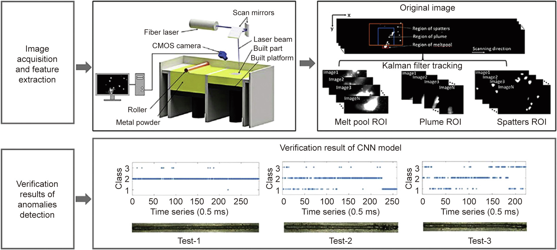
Fig. 3. Scheme of the SLM process monitoring configuration. A high-speed camera is used to capture sequential images of the built process; a CNN model is applied to identify quality anomalies. CMOS: complementary metal-oxide semiconductor; ROI: region of interest. Reproduced from Ref. [37] with permission of Elsevier, ©2018.
《3.3. Process–property–performance linkage》
3.3. Process–property–performance linkage
From a technological and economic point of view, process parameter selection for the optimization of the performance of AM parts is highly desirable. Constructing a direct linkage between process, property, and performance is of great interest to scientists and engineers. This linkage is often highly nonlinear, since the amount of the input variables is usually greater than three. As a result, it is very difficult to identify the underlying mathematical formula for such a linkage. Because of its intrinsic nonlinear characteristics, NN models have been applied to formulate these mathematical relationships for various AM processes. Table 1 [39–55] summarizes the application of NNs into AM (in fact, NN is referred to here as MLP, since all the datasets are the tabular type), and lists the input values of the processing parameters and the output values of the property/performance. As can be seen in Table 1, different AM techniques should select different input features, since the key factors in determining the AM part are different. Furthermore, because a large number of parameters can exert influence on the final products, determining which parameters to select requires a deep knowledge of the AM process. This topic will be discussed in detail in Section 4.3.
《Table 1》
Table 1 NN application to build process–property–performance linkage.

SL: stereolithography; LMD: laser metal deposition; WAAM: wire and arc additive manufacturing.
The detailed setting of the NN algorithm is summarized in Table 2. The typical hyperparameters to determine an NN structure usually consist of four parts: the number of hidden layers, number of neurons in one layer, activation function, and loss function.
(1) Number of hidden layers. In the ‘‘Layer/neuron” column of Table 2, ‘‘5-8-1” means that this NN contains three layers: the input layer has five neurons, the only hidden layer has eight neurons, and the output layer has one neuron. As can be seen from the table, one hidden layer is sufficient for a large majority of AM problems.
《Table 2》
Table 2 Detailed information on the NN algorithm.

MAE: mean absolute error; RMSE: root mean square error; SSE: sum square error.
(2) Number of neurons in one layer. The neuron numbers of the input layer and output layer are determined by the problem itself. However, the number of neurons for the only hidden layer needs to be selected carefully, since it is directly related to the underfitting and overfitting problems in ML [56]. According to Table 2, we suggest 5–10 neurons to be the starting point for determining the optimal number of hidden units for AM applications.
(3) Activation function. The activation function is the nonlinear transformation over the input signal (x); it decides whether a neuron should be activated or not. This is of vital importance to the NN, because a network without an activation function is just a linear regression model, and cannot handle complicated tasks. Some popular types of activation functions are as follows:

In a real implementation, the gradient toward either end of the sigmoid and tanh functions and at the negative axis of the ReLU function is going to be small and even zero; as a result, the weights will not be adjusted during learning. This situation gives rise to the vanishing gradient problem. Max–min normalization, which refines the inputs to a range 0ð Þ ; 1 , is a good supplementary technique to avoid this problem. If necessary, batch normalization [57] should be used in order to continue to refine input signals in every layer.
(4) Loss function. The loss function should be determined by the exact problem, and often carries a real-world interpretation. For example, both the root mean square error (RMSE) and the mean absolute error (MAE) are ways of measuring the distance between two vectors: the vector of predictions and the vector of target values. Their expressions are listed below:

where  is the sample index,
  is the predicted value, and
  is the targeted value. There are some small variations between them: Computing the RMSE corresponds to the
  norm (i.e., the Euclidean norm), which is the most common familiar distance; computing MAE corresponds to the
  norm (i.e., the Manhattan norm), which measures the distance in a rectangular grid from the origin to the target. More generally, the
  norm is expressed by the following:

where  is the norm index. The bigger is, the more sensitive it is to large values. For example, since an norm squares the error, the model will encounter a much larger error than the norm. If this case is an outlier, the norm will pay more attention to this single outlier case, since the errors of many other common cases are smaller. In other words, if it is important to consider any outliers, the RMSE method is a better choice. On the other hand, the MAE is more helpful in studies in which outliers may safely and effectively be ignored. It should be noted that in some special cases, it may be necessary to consider designing the loss function in house.
《4. Challenges and potential solutions》
4. Challenges and potential solutions
《4.1. Small dataset》
4.1. Small dataset
Since the NN method is data-driven, its performance is directly related to the amount of accessible data. Some areas have built their own big datasets for training, such as ImageNet [58] for image recognition, MNIST [59] for optical character recognition, SQuAD [60] for natural language processing, and YouTube-8M [61] for video classification. As a result, NNs have demonstrated their great power in these areas. In contrast, AM has no huge dataset, as it is always expensive to collect training data. Furthermore, economic considerations limit the activity of interested parties to create their own open-source dataset. As a result of this dilemma, it is essential to build up the current small datasets. In fact, certain methods called generative models can realize data augmentation in order to enlarge a dataset artificially. For example, the autoencoder is a representative technology that is capable of randomly generating new data that looks very similar to the training data [11]. It uses an encoder to convert the inputs to an internal representation, and then uses a decoder to generate new outputs that are similar to the inputs based on this representation. A famous extension of the basic autoencoder is called the variational autoencoder (VAE) [62]. It transforms the input into a Gaussian distribution with mean  and standard deviation
  ; when the decoder samples a point from this probabilistic distribution, new input data generates. Other generative models, such as generative adversarial nets (GANs) [63] and adversarial autoencoders (AAEs, in a combination of AE and GAN) [64], can also provide ways to perform data augmentation.
《4.2. Lack of experience in labeling data》
4.2. Lack of experience in labeling data
As mentioned before, most of the NN use-cases are supervised learning, which requires outputs as targets to learn. However, sometimes it is very difficult to label data. For example, how can the different objects in Fig. 3 be accurately labeled as melt pool, plume, or spatters? The authors of Fig. 3 admit that many spatters have characteristics that are similar to those of a melt pool in terms of shape, size, and grey value. In other words, these judgments heavily rely on the analyst’s deep knowledge of the welding process. Such a dependency will greatly hinder the development of NNs in the AM area. In other words, the massive application of NNs to AM requires deep cooperation between experts in both computer science and material science.
《4.3. Lack of knowledge in selecting good features》
4.3. Lack of knowledge in selecting good features
Many processing parameters may heavily affect the properties of AM parts, whereas others may have a smaller effect. Meanwhile, for a limited dataset, an overabundance of input features can easily cause the model to overfit. Therefore, it is of vital importance to ensure that the NN algorithm is operating on a good set of features. A type of preprocessing on input data named feature engineering can bring considerable benefits to researchers. It can be divided into two aspects: ① Feature selection aims to select the most useful features from the existing ones as inputs. For example, people may select ‘‘hatch distance,” ‘‘laser power,” and ‘‘layer thickness” as the most influential factors in determining the properties of parts. In this situation, the principles of selection rely on the researchers’ experience with and knowledge of AM—that is, in terms of performing in-depth investigation into the mechanisms of the AM process, not just in terms of doing experiments again and again. Another useful way is to use statistical tools to perform quantitative analysis. The following are some widely used parameters in statistical science. The Pearson correlation coefficient is a good parameter to measure the linear relationship between two features; when it is close to 1/-1, it indicates that there is a strong positive/negative correlation between these two inputs. The Kendall rank correlation coefficient is another parameter to measure the nonlinear relationship between two features. A scatter matrix is a mathematical tool to plot every numerical attribute against every other numerical attribute. Through the calculation of these parameters, it is possible to obtain information on which attributes are much more correlated with the targeted property. ② Feature combination aims to perform dimensionality reduction on input features, and thus concentrates on newly produced features. Once the translation rule is known, manual manipulation may be preferable. For example, energy density has been shown to have an obvious influence on solidification and metallurgy during AM processing, as well as on the resulting microstructures and mechanical properties of the fabricated parts [65]. Energy density  is represented in SLM as follows:

where  is laser power,
  is scan speed,
  is hatch distance, and
  is layer thickness. These four features can then be converted into the novel but influential feature
  . Furthermore, it is still possible to use mathematical tools for assistance, such as applying principle components analysis (PCA) to reduce dimensionality based on the feature’s value rather than its attribute.
《4.4. The problem of overfitting and underfitting》
4.4. The problem of overfitting and underfitting
A good generalization ability is the key goal of an NN algorithm, and is a measure of how accurately the algorithm is able to predict outputs from previously unknown data. However, a cause of poor performance of an NN algorithm is the overfitting or underfitting problem. Overfitting means that the NN algorithm tries to fit every data point in the training set; thus, the model is very vulnerable to noises or outliers. In contrast, underfitting means that the NN algorithm fails to extract the reasonable relationship between the data points in the training set. Some techniques to avoid overfitting and underfitting include regularization [66] and dropout [67].
《5. Future perspectives》
5. Future perspectives
《5.1. Data》
5.1. Data
5.1.1. Strengthening the interoperability of APIs for data acquisition
With the rapid development of AM, huge amounts of data are generated every day. However, the accessibility of these data is not easy across different research groups, since the data in ‘‘these isolated islands” usually have inconsistent application programming interfaces (APIs) to call. Thus, a unified API for data acquisition will be beneficial for every stakeholder in this area. The paradigm for this kind of qualified API should include welldefined schema for the thermal–mechanical attributes and processing parameters of materials, a unified image type for microstructure characterization, and the same testing standards for qualification. In this way, there will be fewer or no barriers to ‘‘fluent” data flow, and a closer e-collaboration will be realized in the community.
5.1.2. Data preprocessing
Data preprocessing is an essential prerequisite for a data-driven NN algorithm, since it erases ‘‘dirty” data and feeds the correct data into the models. However, this step usually includes many cumbersome tasks that need to be accomplished. For example, there is currently a batch of scanning electron microscope (SEM) images that contain both grain and porosity information, while the corresponding NN model only requires the crack feature as inputs. The problem is to accurately extract the crack distribution separately from the grain boundaries. It can be a challenge for someone without solid knowledge and experience in image processing and analysis to identify these digital representations of structural features. One necessary task may be to establish standards and best practices for data preprocessing, especially for image features. A successful implementation can then be transferred to a broader area.
5.1.3. Database construction
In many material areas, researchers have developed wellknown databases for organizing/storing/accessing data electronically, such as MatWeb, OQMD, and Citrine [68]. Given the high complexity and variety of AM, it is necessary to build a unified database platform to host the huge amounts of data that are generated every day by different research groups and different machines. A currently accessible project is the AM Material Database (AMMD), which was developed by the National Institute of Standards and Technology (NIST) [69]. This data management system is built with a Not Only Structured Query Language (NoSQL) database engine, whose flexible data structure fits the AM case very well. AMMD is web-visualized by the Django framework, so it is very easy to access. For application development, AMMD also provides a representational state transfer (REST) API for third parties to call.
《5.2. Sensing》
5.2. Sensing
5.2.1. Hardware
As demonstrated in Section 3.2, researchers have developed several kinds of sensor systems in order to provide real-time information on AM. Sensors are deployed to precisely detect and measure optical, thermal, acoustic, and ultrasonic signals, and to deliver valuable insights to solidify the understanding of AM. However, huge requirements still exist for a reliable sensor system. For example, the sensors installed inside of a printer must survive and operate in a harsh environment for a long time. In EBM technology, the metallic vapor generated by a high-energy electron beam in a vacuum environment may destroy the camera lens. Furthermore, the sensor system must be quick enough to capture the central position of the melt pool, since the laser’s scanning speed is usually very fast. From this perspective, a qualified sensor system is highly desirable in the rapid developing area of AM.
5.2.2. Software
The sensors need to be controlled by powerful operating software. The basic modes of the control software include monitoring, recording, analyzing, and storing data. In a typical scenario, such as during the process of SLM, once the hardware delivers the captured melt pool image to the software, it may have the capability to compute the temperature profiles and extract thermal and dimensional metrics for next-step analysis. Other interesting functional points can be added to the sensing software. For example, it is desirable for software to be equipped with the algorithms of detecting voids, lack of fusion or porosity, and so forth (especially aided with ML methods).
《5.3. Control/optimization》
5.3. Control/optimization
AM builds parts layer by layer, and the quality of every layer exerts a great influence on the properties of the final products. As a result, it is necessary to ensure the quality of every layer. Multiple types of sensors, such as those capturing photonic, electrical, sonic, and thermal signals, can provide in situ measurements of the AM process. Closed-loop control can be achieved with the application of ML in order to analyze this information synchronously and then feed the outputs into the controller of the machine. A possible use is to train a CNN to judge whether the quality of a layer is adequate or not based on the layer picture captured by a high-speed camera. In this case, the NN algorithm must quickly respond to the input picture. Fortunately, some model compression technologies are already available, such as parameter pruning and sharing, low-rank factorization, and knowledge distillation [70].
《5.4. Whole chain linkage》
5.4. Whole chain linkage
Sections 3.2 and 3.3 have shown the great power of NNs in building the relationships between structure–property and process–property, respectively. In addition, researchers have constructed other models to establish the process–structure– property–performance (PSPP) linkage. For example, Azimi et al. [71] utilized a fully convolutional neural network (FCNN) to classify martensite/bainite/pearlite phases in low-carbon steels, as depicted in Fig. 4. The classification accuracy can reach 93.94%, which greatly exceeds the state-of-the-art method with an accuracy of 48.89%. Although this case is not within the scope of AM, its concept can easily be transferred to AM; we anticipate an explosive development in building PSPP linkages using NNs, since the latter holds intrinsic advantages in complex pattern recognition in comparison with other methods and models.
《Fig. 4》
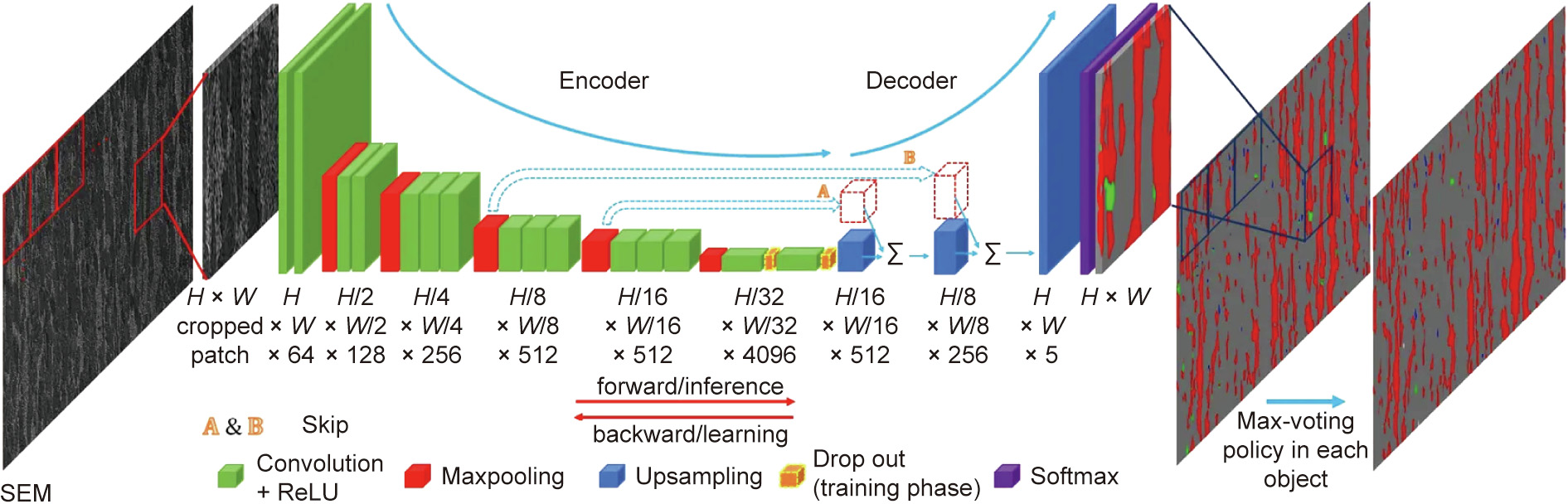
Fig. 4. Workflow of martensite/bainite/pearlite classification approach using FCNNs. H: height; W: width. Reproduced from Ref. [71] with permission of Springer Nature,© 2018.
《5.5. Modeling forecasting》
5.5. Modeling forecasting
As mentioned before, the physics-based model is a traditional computational way to reproduce the AM process. However, it requires substantial computational cost in terms of time, hardware, and software. As demonstrated in Section 3.1, it is possible to learn from previously accumulated numerical datasets and extract the embedded linkages between inputs and simulated outputs. In other words, numerical simulations can be a data source for the ML algorithm, and can play the same role as experimental data. Popova et al. [72] developed a data science workflow to combine ML with simulations. This workflow is then applied to a set of AM microstructures obtained using the Potts kinetic Monte Carlo (kMC) approach, which is open-source hosted in the Harvard Dataverse [73]. Karpatne et al. [74] proposed the concept of theory-guided data science (TGDS) as a new paradigm for integrating physics-based models and data-driven models. They have identified five broad categories of approaches for combining scientific knowledge with data science in diverse disciplines. In the near future, the combination of these two kinds of models will certainly provide a way to address the current issues of a lack of experimental AM data, non-interpretable NN models, and so on.
《6. Conclusion》
6. Conclusion
Two explosive developments have recently occurred in the areas of manufacturing and information technology: AM and NNs. AM has advantages such as integration with digital CAD models and the capability to build parts with complex morphology, while NNs excel at avoiding constructing and solving complicated multiscale and multi-physical mathematical models. The combination of AM and NN has demonstrated great potential for realizing the attractive concept of ‘‘agile manufacturing” in industry. This paper provided a comprehensive overview of current progress in applying the NN algorithm to the complete AM process chain, from design to post-treatment. The scope of this work covers many variants of NNs in various application scenarios, including: a traditional MLP for linking the AM process, properties, and performance; a convolutional NN for AM melt pool recognition; LSTM for reproducing finite-element simulation results; and the VAE for data augmentation. However, as they say, ‘‘every coin has two sides”: It is difficult to control the quality of AM parts, while NNs rely strongly on data collection. Thus, some challenges remain in this interdisciplinary area. We have proposed potential corresponding solutions to these challenges, and outlined our thoughts on future trends in this field.
《Compliance with ethics guidelines》
Compliance with ethics guidelines
Xinbo Qi, Guofeng Chen, Yong Li, Xuan Cheng, and Changpeng Li declare that they have no conflict of interest or financial conflicts to disclose.


 京公网安备 11010502051620号


