Artificial Intelligence in Steam Cracking Modeling: A Deep Learning Algorithm for Detailed Effluent Prediction

Abstract

Chemical processes can benefit tremendously from fast and accurate effluent composition prediction for plant design, control, and optimization. The Industry 4.0 revolution claims that by introducing machine learning into these fields, substantial economic and environmental gains can be achieved. The bottleneck for high-frequency optimization and process control is often the time necessary to perform the required detailed analyses of, for example, feed and product. To resolve these issues, a framework of four deep learning artificial neural networks (DL ANNs) has been developed for the largest chemicals production process—steam cracking. The proposed methodology allows both a detailed characterization of a naphtha feedstock and a detailed composition of the steam cracker effluent to be determined, based on a limited number of commercial naphtha indices and rapidly accessible process characteristics. The detailed characterization of a naphtha is predicted from three points on the boiling curve and PIONA (paraffin, isoparaffin, olefin, naphthene, and aromatics) characterization. If unavailable, the boiling points are also estimated. Even with estimated boiling points, the developed DL ANN outperforms several established methods such as maximization of Shannon entropy and traditional ANNs. For feedstock reconstruction, a mean absolute error (MAE) of 0.3 wt% is achieved on the test set, while the MAE of the effluent prediction is 0.1 wt%. When combining all networks—using the output of the previous as input to the next—the effluent MAE increases to 0.19 wt%. In addition to the high accuracy of the networks, a major benefit is the negligible computational cost required to obtain the predictions. On a standard Intel i7 processor, predictions are made in the order of milliseconds. Commercial software such as COILSIM1D performs slightly better in terms of accuracy, but the required central processing unit time per reaction is in the order of seconds. This tremendous speed-up and minimal accuracy loss make the presented framework highly suitable for the continuous monitoring of difficult-to-access process parameters and for the envisioned, high-frequency real-time optimization (RTO) strategy or process control. Nevertheless, the lack of a fundamental basis implies that fundamental understanding is almost completely lost, which is not always well-accepted by the engineering community. In addition, the performance of the developed networks drops significantly for naphthas that are highly dissimilar to those in the training set.

Content

《1. Introduction》

1. Introduction

With the majority of light olefins being produced via steam cracking—both today and in the foreseeable future [1]—it is important to take advantage of new technological developments and innovations in this field. One such development that has taken the world by storm in the past few years is artificial intelligence (AI). AI has been widely adopted in several fields such as strategic gaming [2,3], natural language processing [4,5], and autonomous cars [6,7]. More recently, AI techniques have found their way into chemical (engineering) research [8]. Slowly but steadily, AI is also making its way into industrial manufacturing and production processes [9]. Admittedly, the bulk chemical industry has been relatively conservative in this transition in comparison with the automotive sector, for example. The upcoming technological revolution has been termed Industry 4.0, and is expected to redefine the limits of production [10–14]. Examples of the use of AI in chemistry include, among others, drug discovery [15,16] and synthesis [17,18], and computational chemistry [19]. As indicated by the examples above, AI techniques excel at tackling highly complex and nonlinear problems. Therefore, application of these methods to the modeling of the reactor section of the steam cracking process, which is itself complex and nonlinear, will deliver models that are expected to outperform traditional detailed kinetic models in both execution speed and accuracy. With the increasing complexity and performance of real-timeoptimization (RTO) systems—both in steam cracking and other industries [20–22]—the necessity for detailed inputs increases as well. While technically feasible, the use of comprehensive, online, two-dimensional gas chromatography (2D-GC or GC × GC) for detailed stream characterization has not found its way into industry [23], due to its labor-intensive and time-consuming data processing. Hence, the detailed compositions required in RTO systems are usually obtained via sampling and offline analyses. These time-consuming analyses result in RTO systems that perform only one optimization step every few hours [24]. The above does not imply that online characterization techniques are not applied in industry; rather, the employed techniques for online characterization often relay much less detailed information than comprehensive GC × GC. Besides their value to RTO, detailed knowledge of reactor input and output compositions is crucial to safe and efficient operation. In addition, the development of accurate reactor models relies heavily on the level of detail of the feedstock and effluent characterization. The above implies the necessity for both feedstock reconstruction and reactor modeling algorithms. There is no lack of research on either of these topics, but few approaches incorporate AI. Hudebine and Verstraete [25], Verstraete et al. [26], and later, Van Geem et al. [27] used entropy maximization methods with great success in feedstock reconstruction of various petroleum fractions. In reactor modeling, the use of increasingly detailed kinetic models dominates other methods due to their capability to extrapolate beyond the ranges of predefined training sets [28–35]. Artificial neural networks (ANNs) are a frequently used AI tool [36]. This form of biomimicry is a simplified mathematical representation of the neural network of the human brain, as illustrated in Fig. 1 [37].

《Fig. 1》

Fig. 1. Analogy between (a) a biological neuron and (b) an artificial neuron or perceptron, after Mahanta [37]. i: inputs; w: weights; o: output; : activation function.

An example of the use of AI on the side of feedstock reconstruction is the work by Pyl et al. [38], who developed an ANN to determine the detailed molecular composition of naphthas typically used in cracking processes, based on their paraffins, iso-paraffins, olefins, naphthenes, aromatics (PIONA) composition and boiling point (BP) curve. Niaei et al. [39] and later Sedighi et al. [40] used ANNs to model reactor effluent compositions, but did so for a given feedstock. Ghadrdan et al. [41] tackled this feedstock hiatus in a qualitative way by introducing a set of nine feed-type parameters to the ANN model. While indisputably powerful tools, traditional ANNs and more classical machine learning techniques rely on the developer identifying the correct features that describe the problem. In this work, a deep learning (DL) approach is applied to the problems of feedstock reconstruction and reactor effluent prediction for naphtha feedstocks. DL further exploits the power of ANNs by relying on the network itself to identify, extract, and combine the inputs into abstract features that contain much more pertinent information to solving the problem—that is, predicting the output, as illustrated in Fig. 2 [42,43]. The idea is that this additional level of abstraction improves the capability of the network to generalize to unseen data and hence outperform traditional ANNs on data outside of the network training set.

《Fig. 2》

Fig. 2. Shallow ANN compared with a DL ANN, after Seif [43]. T: temperature; P: pressure; E/E: the product ratio of ethylene to ethane; P/E: the product ratio of propylene to ethylene; M/P: the product ratio of methane to propylene; Y₁: output 1; Y₂: output 2; Y₃: output 3; a: certain value; : activation function.

In what follows, four interacting DL ANNs are described, with achieving predictive accuracy on the steam cracker reactor effluent composition as the final goal, using a limited number of commercial indices of the feedstock as input. Fig. 3 illustrates this interacting DL ANN framework. Network 1 uses the most basic inputs—PIONA, density, and vapor pressure—as input to predict the initial boiling point (IBP), mid boiling point (BP50), and final boiling point (FBP). Network 2 uses these predicted BPs, in combination with the previously specified PIONA, to make a detailed reconstruction of the feedstock, which can then be used as input to Network 3. This network predicts a detailed composition of the effluent. Network 4 serves as an extension and check for Networks 1 and 2. Using a detailed PIONA characterization of a naphtha, it predicts its density, vapor pressure, and the three aforementioned BPs.

《Fig. 3》

Fig. 3. Schematic overview of the interaction of the different variables and the four networks in the DL ANN framework. The numbers in brackets refer to the number of descriptors for each variable.

Before presenting the architecture of the individual DL ANNs in Section 3, the theory of ANNs is briefly discussed and some comments concerning the data are given in Section 2 and in Supplementary data. In Section 4, the results of the trained networks are discussed and compared with those of other reconstruction and prediction methods, including support vector regression (SVR) and random forest (RF) regression. In the final section, we give a brief summary and comment on future prospects of this promising approach for steam cracking effluent prediction.

《2. Methods and data》

2. Methods and data

《2.1. Deep learning artificial neural networks》

2.1. Deep learning artificial neural networks

The mathematical aspects of (DL) ANNs are similar; therefore, no distinction will be made in this section between traditional ANNs and DL ANNs [44]. The relationship between the input vector and output o of a single perceptron is given by Eq. (1). All inputs are weighted by their respective weights and then summed. A constant bias term b is added to this weighted sum. The activation function introduces nonlinearity into the network. Commonly used activation functions are the sigmoid, hyperbolic tangent, rectified linear unit (ReLU), and softmax functions. More information on these activation functions can be found in Section S1.1 in Supplementary data. The equation for a single perceptron is easily extended to Eq. (2) to describe a full layer of the network, where W is the weight matrix of the layer. Each perceptron can have its own bias parameter. The entire network is finally described mathematically by repeatedly applying Eq. (2), which yields Eq. (3) for an ANN with one input layer, one hidden layer with bias b₁, and one output layer y with bias b₂.

where w is the weight vector for a single perceptron; i is the input to the perceptron; j is the node index within the layer.

where o is the layer output vector.

where y is the model output vector; x is the model input vector; and are the activation functions for layer 1 and layer 2, respectively; are the bias vector for layer 1 and layer 2, respectively.

The ANNs in this work are trained via back-propagation algorithms [44,45], which update the network layer weights by passing down the error from one layer to the next, starting at the output. A gradient descent optimization approach is used to minimize a certain objective function. Frequently used error metrics in the objective function are the (root) mean squared deviation (RMSD), mean absolute error (MAE), and mean absolute percentage error (MAPE). Several iterations through the complete training set are typically required to optimize the weights. One such iteration is termed an epoch. Within one epoch, the training set is further split into several batches. The network weights are updated once per batch. A small batch size—that is, a limited number of samples per optimization step—results in faster training in terms of the number of required epochs, but slower training in terms of computing time per epoch. Moreover, a smaller batch size results in poorer gradient estimates, reducing the stability of the optimization.

In ANNs, a distinction can be made between overfitting and overtraining of the network [46]. Overfitting occurs when the network becomes too complex—that is, when too many layers or too many nodes per layer are used. According to the universal approximation theorem, for any function, an ANN can be found that approximates the data with any desired accuracy [47]. Overtraining, on the other hand, pertains to the number of training epochs. If the training data is shown to the network too often, it will start “memorizing” the data; that is, it will attempt to predict the exact output values, rather than the ones expected from the generalized trend in the data. This is illustrated by a simple example. Assume two variables are linearly related. In the dataset, one data point does not follow this linear trend, for example due to a measurement error. After a few training epochs, the network will have recognized the linear trend. The sum of squares, however, is still high due to the off-trend data point. During training, the sum of squares is minimized. As a result, in each subsequent epoch, the network will start describing a trend that is increasingly less linear, because after seeing the off-trend data point multiple times, it “believes” that that point is on-trend too. Overtraining can be ascertained by monitoring the objective function or network accuracy of both the training and validation datasets. While for the training set, the objective function will typically follow a decreasing trend with an increasing number of epochs, the objective function for the validation data will start to increase again at some point. From this point onward, the network is being overtrained. The above issues can be remedied, for example, by using dropout during training [48,49]. In this technique, during each batch of data, a randomly selected fraction of the network nodes is temporarily eliminated from the network. In this way, each neuron must individually learn characteristics—it cannot rely on neighboring neurons to capture information. All networks in this work use a dropout ratio of 0.5. The tradeoff for the reduced overfitting with dropout is that the network learns more slowly, as only half the weights are updated in each step. Other regularization techniques such as L1 and L2 regularization [50] of the objective function have not been evaluated in this work, as the constructed networks perform well on the test data.

《Fig. 4》

Fig. 4. (a) Eigenvalues and explained variance (the percentages above data point) by the principal components (PCs); (b) decomposition of the inputs along the first and second PCs (score plot); (c, d) PC representation of the naphtha test set, with outliers indicated in red. P: paraffins; I: iso-paraffins; O: olefins; N: naphthenes; A: aromatics.

The python deep learning library Keras [51], with Tensorflow backend [52] and graphics processing unit (GPU) acceleration, is used to train the ANNs.

《2.2. Data analysis》

2.2. Data analysis

2.2.1. Naphthas

The work of Pyl et al. [38] provides a set of 272 detailed industrial naphtha compositions. The available naphtha properties include density, vapor pressure, three BPs determined via the ASTM D86 standard method—IBP, BP50, and FBP—and detailed PIONA fractions per carbon number. Fig. S13 provides a correlation matrix of the available data. It can be observed that vapor pressure and IBP are strongly correlated, as are the density and BP50. The FBP is less strongly correlated to density and vapor pressure, but significant correlation to the BP50 is present. This correlation will influence the architecture of the network to predict the BPs from the vapor pressure and density of the naphtha, which will be discussed in Section 3.1.

Along the same lines as the work by Pyl et al. [38], a principal component analysis (PCA [53]; details in Section S1.2) is performed on the 10 input variables of the dataset: IBP, BP50, FBP, density, vapor pressure, and PIONA. Fig. 4 summarizes the PCA results. From Fig. 4(a), it can be concluded that the (training) dataset is described by three components. The scores of the inputs on the first two of these principal components (PCs), shown in Fig. 4(b), confirm the findings from the correlation analysis. The high correlation observed between, for example, density and BP50 translates into parallel vectors in the PC space. Although they have opposite directions, the IBP and vapor pressure present similar behavior.

A second analysis based on PCA is performed on the test set. As ANNs rely only on the training and validation datasets during training, it can be expected that only test data that resembles the training and validation data will yield accurate results. One measure to determine the resemblance of a data point to the training set is the Mahalanobis distance (MD) [54,55]. In the PC space, the MD can be calculated via Eq. (4).

where represents the input in the PC space and contains the scores of the original input on each of the PCs. is the diagonal matrix of all eigenvalues, which in this case is a 10 × 10 matrix. is the reduced 3 × 3 eigenvalue matrix, and contains only the eigenvalues corresponding to the three selected PCs. Naphthas with a high MD can be considered outliers, and can hence be expected to result in poorer predictions. Figs. 4(c) and (d) indicate the test set distribution in the PC space. The dotted line corresponds to a MD of 2.5 and represents a probability of 90% that a naphtha situated within the ellipsoid is within the range of the training set. This value of 2.5 for the MD is used as critical distance to consider whether the corresponding naphtha is an outlier or not. One naphtha (indicated in red in Fig. 4) has a MD of 5.08. In conclusion, this analysis indicates that the predictions should be good in general, but may be off for the aforementioned naphtha.

2.2.2. Effluent composition

Access to detailed industrial steam cracker effluent compositions is highly restricted. Therefore, the state-of-the-art reactor simulation software tool COILSIM1D by Van Geem et al. [30,56] and Vervust et al. [57] was used to obtain the required effluent characterizations. COILSIM1D has been validated against large amounts of proprietary data and is used in industry for detailed steam cracker simulations; thus, it is a reliable and accurate tool, and the obtained results are trusted to be an adequate replacement of the unavailable experimental or industrial data. This approach of using simulation data as replacement for unavailable and/or limited experimental data has become common practice in other fields, especially in the prediction of the thermodynamic properties of molecules and reaction kinetics [58–63]. The use of simulated data as training data, the difficulty in obtaining experimental data, and the necessity of accurate input and output data underline both the continuing importance of detailed, fundamental models for the simulation and understanding of these processes and the critical necessity for high-accuracy experimental techniques.

COILSIM1D can predict up to hundreds of individual chemicals in the output. The majority of these components, however, are of minor importance to the overall operation of a steam cracker. Therefore, 28 (pseudo-)components are identified. These comprise several molecular components such as ethylene, propylene, benzene, hydrogen, and butadiene, and lumped components such as C₇ iso-paraffins and C₁₀₊ aromatics. The full list of components can be found in Section S2. Two sets of simulations are run.

The first set comprises a total of 13 600 simulations, and is used to train and test the network to predict detailed effluent compositions. A different naphtha composition is used for each simulation. The different naphtha compositions are obtained from the dataset described in Section 2.2.1, but random variations of 0%–10% are introduced into the concentrations. Each naphtha is combined with a set of different process conditions. These process conditions are the coil outlet pressure (COP) and coil outlet temperature (COT). Fig. S14 shows that both the naphtha compositions and process conditions cover a wide range of the variable space in a uniform way. A single reactor and furnace configuration are used for all simulations. It will be shown later that the exact reactor configuration is of minor importance. A PCA on the new dataset is performed to identify potentially problematic cases. Fig. 5(a) indicates that the dataset is described well by six PCs. When projecting the test dataset onto the first three dimensions of the PC space, as shown in Fig. 5(b), a small amount of inputs are observed to be situated outside of the ellipse encompassing 90% of the training data and corresponding to a MD of 3.3. Again, this indicates that good overall performance on the test set can be expected, with a limited number of poor predictions.

The second set consists of 1587 additional simulations and is used to test the full workflow and combined performance of the networks. The same reactor and furnace configurations as for the previous simulations are used. A total of 32 naphtha compositions are considered in this set, corresponding to the test set of Networks 1, 2, and 4, such that no training data is ever used during testing. Each of these naphthas is extended by a set of process conditions in fixed intervals. In the range between 750 and 950 °C, 10 COTs are considered. Similarly, five COPs between 1.7 and 2.3 bar (1 bar = 10⁵ Pa) are accounted for. Although this results in a somewhat grid-like coverage of the variable space, it is sufficient for testing purposes.

《Fig. 5》

Fig. 5. (a) Eigenvalues and explained variance for the first 20 PCs in the PCA of the effluent dataset; (b) effluent test data in the PC space reduced to three dimensions.

《3. Setup of the ANNs》

3. Setup of the ANNs

《3.1. From density and vapor pressure to BPs》

3.1. From density and vapor pressure to BPs

The aim of this work is to develop a set of algorithms that allow a user to obtain a detailed prediction of the steam cracking reactor effluent, using only readily available descriptors. As detailed predictions are more reliable when using detailed feedstock characterizations, a first step in the algorithm is reconstructing the feedstock from its commercial descriptors. Based on previous work by Van Geem et al. [27,30–32] and Pyl et al. [38], it is apparent that at least some points on the naphtha BP curve are required in order to successfully reconstruct the naphtha composition. However, BPs are difficult to measure online, as a single ASTM 86-compliant measurement can take 30–45 min [64]. Thus, they are not considered to be readily available. Therefore, estimating three important points on the BP curve is the first useful step toward predicting the effluent composition. The prediction of the BPs is based on the density, vapor pressure, and basic PIONA characterization of the naphtha. Based on the (cor)relations between the feed parameters described in Section 2.2.1, a network is constructed, the architecture of which is shown in Fig. 6. Due to the strong correlation of both the IBP and BP50 with the FBP, the vector containing the estimates for the IBP and BP50 is concatenated with the first hidden layer. This allows the network to use the predictions for the IBP and BP50 directly during the prediction of the FBP. The first hidden layer is chosen over the input layer because in the DL approach, the network is considered to learn the most relevant representation of the input toward predicting the output in this first hidden layer. Henceforth, this network will be referred to as Network 1. To increase the stability and performance of the network, all inputs and outputs are normalized to the range of the dataset. The maxima and minima on which each variable is normalized are listed in Table 1. The dataset of 272 naphthas is split into training, validation, and test sets according to an 80:8:12 split. The validation set is used to tune the hyperparameters of the network—in this case, the number of nodes in the hidden layers, the batch size, the activation functions, and the number of training epochs. In general, the term hyperparameters denotes all parameters of the network except for the node weights and biases, which are referred to as the network parameters. The optimal combination is searched for heuristically. More detailed information on this search is given in Section S3.1. The test set is used for evaluation of the final optimized network.

《Fig. 6》

Fig. 6. Architecture of Network 1, for predicting the IBP, BP50, and FBP, based on the PIONA composition, vapor pressure, and density of the naphtha.

《Table 1》

Table 1 Range for input and output variables of Network 1.

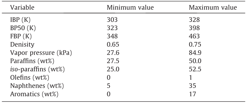
The resulting hyperparameters are shown along with the architecture in Fig. 6. Additional figures comparing the performance of the network with different hyperparameters can be found in Section S3.2. The MAE is preferred to the mean squared error as the training objective function because, given the considered hyperparameter grid (Section S3.1), the finally chosen network is observed to have the lower mean squared error. A detailed explanation for this specific network is given in Section S3.2. Due to the normalization of the individual components, all outputs are of a similar order of magnitude. The use of the MAPE is therefore not considered to be beneficial to the network accuracy. The best performance in terms of MAE is achieved with a batch size of 8, after 1181 training epochs. The final network—using the optimized hyperparameters—is trained on both the training and validation data, after which the network is validated against the unseen test data.

《3.2. Feedstock reconstruction》

3.2. Feedstock reconstruction

The second network in the framework uses the PIONA composition of the naphtha and the BPs to reconstruct the detailed composition of the feedstock. For training the network, the experimental BPs are used as input. In line with the work of Pyl et al. [38], 28 different pseudo-components are estimated, corresponding to the detailed PIONA matrix in Fig. S15. An additional distinction is made between xylenes and ethylbenzene, and between cyclohexane and methyl-cyclopentane in the A₈ and N₆ categories, respectively. The inputs are normalized along the same procedure as in the previous section, with the ranges listed in Table 1. For the outputs, a different normalization procedure is applied. The absolute concentrations of the components in the different categories span a very wide range. The mass fraction C₅ and C₆ components can be as high as 35 wt%, while the olefin fraction can drop to 0.01 wt%. Attempting to directly predict all fractions at once, with a single softmax function, will result in a network that is difficult to train, especially considering the limited amount of available training data. The benefit of using a single softmax layer is that the outputs sum to one, corresponding to the physical nature of the desired mass fractions. Due to the wide range in mass fractions, however, the five PIONA categories in the output are normalized individually according to the example for the paraffins in Eq. (5).

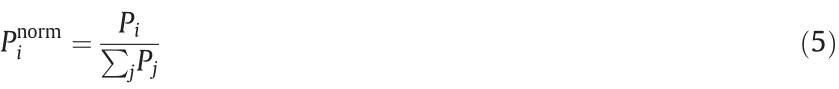
where represents a normalized PIONA category; is a PIONA category.

By first splitting the output layer into five separate outputs, a softmax activation function can be used for each individual component category, with the exception of the olefin mass fraction. Due to the fact that the total olefin concentration can be zero, and according to the nature of the softmax activation function, the network is forced to incorrectly predict an olefin distribution that sums to one. This has a detrimental effect on the overall accuracy. Hence, for the olefin output layer, a sigmoid activation is used. The resulting multi-output architecture and optimized hyperparameters are shown in Fig. 7. In what follows, this network is referred to as Network 2. Again, a train/validation/test split of 80:8:12 is used on the data. Section S3.3 of the supplementary data provides additional details on the optimization. In short, the MAE is chosen as the network objective function. Due to the normalization per component class, the outputs do not span several orders of magnitude and hence do not require a relative cost function. For this network, optimum performance is attained using a batch size of 16 and 45 285 training epochs.

《Fig. 7》

Fig. 7. Architecture of Network 2, for reconstructing a more detailed feedstock composition starting from the PIONA characterization and BPs.

《3.3. Detailed effluent prediction》

3.3. Detailed effluent prediction

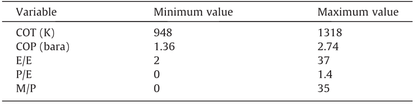
The third network takes a detailed PIONA composition (28 pseudo-components) and five process characteristics as input to predict a detailed molecular composition of the steam cracker reactor effluent. As mentioned in Section 2.2, an adapted dataset is used for this network that contains 50 times more data points than the set used for the previous networks. The components considered in the detailed PIONA composition are the same as in Fig. S15. Based on previous work by Van Geem et al. [31], five process descriptors are identified. The first two—COT and COP— have already been used for the generation of the dataset. The remaining three are the product ratios of ethylene to ethane (E/E), propylene to ethylene (P/E), and methane to propylene (M/P). In the work of Van Geem et al. [31], it is proven that for a given naphtha, the effluent composition is fully defined by just two of these descriptors. However, Fig. S16 reveals that a more accurate model is obtained when all five descriptors are included in the input. Three contributions to this increase in accuracy can be identified. First, by using the aforementioned product ratios as input, the model must predict three fewer outputs, as the methane, ethane, and propylene mass fractions can be calculated from the prediction of the ethylene mass fractions. Second, by including multiple descriptors that essentially describe the same process parameters of temperature and pressure, the model becomes robust to errors in the input, as the uncertainty is spread over multiple inputs. The third and most important reason can be traced back to the power of DL networks, as illustrated in Fig. 2. By training the multilayer network on multiple inputs, it is given the freedom to extract the information from the inputs that it finds to be most pertinent to solving the presented problem of predicting the effluent composition. Training the model using only, for example, COT and COP does not make full use of the potential of DL. By manually selecting or engineering the network inputs and eliminating certain process descriptors from the network input, potentially useful information in the data is never shown to the network. In conclusion, all five identified descriptors are included in the network input.

The values for COT, COP, E/E, P/E, and M/P are normalized on the ranges given in Table 2. Due to a mismatch in size between the inputs, the first layer is split into a process and a feedstock feature layer, yielding a more advanced DL ANN than the regular densely connected ones. This split allows for the extraction of independent, equally long, relevant feature vectors for both inputs. As it is not the complete effluent spectrum that is predicted by the network, the sum of the outputs should not equal one. Hence, a softmax activation function cannot be applied in the output layer and a sigmoid activation is utilized instead, taking into account that the component fractions are bounded by zero and one. The final architecture and hyperparameters are shown in Fig. 8. In this case, the MAPE is chosen as the objective function. Justification for this choice is given in Section S3.4. This network is further referenced in this work as Network 3. For this dataset, a train/validation/test split of 81:9:10 is applied. The network reaches the best performance using a batch size of 8 and 2744 training epochs. Additional information on the optimization of the hyperparameters is given in Section S3.4.

《Table 2》

Table 2 Range for process-related input variables of Network 3.

《Fig. 8》

Fig. 8. Architecture of Network 3, used to predict the molecular effluent composition based on the detailed feedstock composition and five process descriptors.

《3.4. Property estimation》

3.4. Property estimation

A final network in the framework serves as a check for the first two. Based on a detailed naphtha composition, the density, vapor pressure, IBP, BP50, and FBP are estimated. The dataset is identical to the one used for the reverse operation by Networks 1 and 2. Given an accurate reconstruction, the predicted properties of a reconstructed naphtha should not differ much from those reported for the true naphtha. One could argue that the best results are obtained by simultaneously optimizing the four networks. However, given the limited size of the dataset, training such a complex network with multiple feedback loops is considered unfeasible at worst and inaccurate and non-generalizing at best. The fourth network—Network 4—has a straightforward, two-layer architecture, with 28 inputs and five outputs, as illustrated in Fig. 9 along with the optimized parameters. For similar reasons as for Networks 1 and 2, the MAE is chosen as the loss function. The 28 inputs are the same components accounted for in the reconstruction algorithm, and are listed in Fig. S15. The sum of the 28 inputs is normalized to one, whereas the outputs are normalized according to the same ranges listed in Table 1. A batch size of 8 and 5385 training epochs are found to yield the best performance. Additional information on the optimization is provided in Section S3.5.

《Fig. 9》

Fig. 9. Architecture of Network 4, to predict naphtha properties from a detailed PIONA characterization.

《4. Results and discussion》

4. Results and discussion

《4.1. Feedstock》

4.1. Feedstock

The performance of the network to predict the IBP, BP50, and FBP is shown in Fig. 10. Overall, the network performs very well, with only two notably poorer predictions, each for a different naphtha. These are indicated in red and green in Fig. 10. The calculated MD for the predictions in red is 1.82, which is below the critical value of 2.5 (Section 2.2.1), so accurate predictions are expected. The cause of this high error is discussed further on. The naphtha to which the green predictions correspond is situated at a MD of 5.08, which corresponds to a probability of 2 × 10^-5 that the hypothesis of it belonging to the training set holds, for an F-statistic with (3, 237) degrees of freedom. The poorly predicted IBP is outside of the normalization range of the output, as shown in Table 1, indicating that the network must predict a value greater than one, which is impossible by the construction of the network. For the other two BPs, however, the model makes very accurate predictions, despite the strong dissimilarity of the naphtha with the training dataset. Three other naphthas have a MD greater than the threshold value of 2.5. The predictions for these naphthas deviate by up to 10 K from the experimental value. This shows one of the pitfalls of DL or any other type of regression: Inputs that are very dissimilar to those in the training set will likely result in poorer predictions.

《Fig. 10》

Fig. 10. Parity plot for Network 1; prediction of the IBP, BP50, and FBP from PIONA, density, and vapor pressure. The points indicated in green are predictions for a naphtha with a Mahalanobis distance of 5.08; those in red are predictions for one of 1.82.

Table 3 [27] shows that the predicted values deviate around 1% or 3 K from the experimental value on average, for all BPs. This finding further substantiates the claim that it was not necessary to consider training the network on the MAPE. The accuracy of the network does not quite match that of experimental methods, such as one with a maximum MAE of (2.2 ± 1.4) K that was reported by Ferris and Rothamer [65]. However, the DL ANN does perform better than the maximization of the Shannon entropy (MSE) approach used by Van Geem et al. [27]. This observation is not unexpected. The majority of the test set that was used, while never seen by the network during training, is situated within the ellipsoid corresponding to a MD of 2.5 or a probability level of 0.9. Therefore, good performance of the network is expected even on the test set. Even for the data points situated outside of this critical ellipsoid, the DL ANN model still performs similarly to the MSE approach. This is supported by their similar maximal deviations.

《Table 3》

Table 3 Statistical metrics of the performance of Network 1 on the test set compared with work by Van Geem et al. [27].

A very high throughput can be achieved with the network: The prediction of the BPs of the 32 test naphthas took 137 ms on a 2.7 GHz Intel i7-6820HQ central processing unit (CPU), or just over 4 ms per naphtha. Unfortunately, an equivalent speed test using the method of Van Geem et al. [27] was not possible, as the estimate of the BPs is reported as part of the feedstock reconstruction; nevertheless, given the combined time of 25 s, the DL ANN can safely be assumed to be faster.

Fig. 11 shows the performance of Network 2 on a selected number of components of the output. Parity plots for all components in the output can be found in Fig. S17. In general, the performance is good over the entire range of concentrations. The network achieves an overall MAE of 0.31 wt%. Two outlying predictions are singled out in red. In Section 2.2.1, a lack of correlation for the I₇ components with any of the other variables was mentioned. When leaving out the naphthas corresponding to the highlighted points, the correlation of the I₇ component group to other variables is found to increase by over 1%. As the left out data accounts for about 0.7% of the data, it can be concluded that they have a significant impact on the lack of correlation. The calculated MD for the naphthas is 2.27 for naphtha A and 1.82 for naphtha B. Therefore, there is no indication that the naphtha compositions are outside of the scope of the training set. The above suggests that it is possible that a measurement error is causing the poor prediction. This possibility is further supported by the fact that nearly all off-trend predictions noticed for other components (e.g., P₄ and P₇) are the result of the same two problematic naphthas. A measurement error for one or more components could also help explain the poor prediction of the FBP of the naphtha highlighted in red in Fig. 10, as it is the same naphtha as naphtha B. This result highlights the critical importance of high-quality input, both for accurately training the network and for obtaining accurate predictions.

《Fig. 11》

Fig. 11. The performance of Network 2 on selected components of the output.

The performance of Network 2 is compared with previous work on feedstock reconstruction by Van Geem et al. [27] and Pyl et al. [38], and with two additionally constructed models; the reconstruction algorithms are based on the following methods: MSE (Van Geem et al. [27]), multiple linear regression (MLR) (Pyl et al. [38]), traditional ANNs (Pyl et al. [38]), SVR, and RF regression. The MLR approach—which is the traditional method—is used as a performance baseline. Table 4 shows the performance of the different models on the individual components of the output. Machine learning techniques such as SVR and (DL) ANNs show significant improvement compared with more traditional methods such as MLR and MSE. Fig. 12 shows the relative model performance in terms of MAE. The DL approach clearly outperforms all other models: Network 2 attains an MAE that is just over half the MLR MAE and still 20% lower than the ANN MAE. Even when using the predicted BPs based on the density and vapor pressure—combining Networks 1 and 2—the DL ANN still performs noticeably better than all other tested models. While the MSE approach has a significantly higher MAE, its advantage is that it relies on a case-by-case optimization—that is, the applicability of the method is less restricted to the range of a certain training set. In terms of required CPU time, the MSE method takes about 25 s to simulate both BPs and reconstruct the detailed composition for the test set. Using Networks 1 and 2, the combined process only requires about one tenth of that time—234 ms—on the same Intel i7 processor mentioned earlier.

《Table 4》

Table 4 MAE (wt%) of different algorithms for the detailed reconstruction of naphthas, based on PIONA and BPs.

MBP: modeled boiling point.

《Fig. 12》

Fig. 12. Network MAE relative to that of the MLR model. DL ANN MBP uses the MBPs as input, with a combined performance of Networks 1 and 2.

Network 4 also pertains to the feedstock, as it estimates properties based on a known, detailed composition. The performance of this network is illustrated by the parity plots in Fig. 13. The singled-out predictions in Fig. 13(a) correspond to those for naphtha B, mentioned above. Again, the poor prediction for the vapor pressure could be the result of measurement errors during the compositional analysis of the naphtha. Table 5 shows the statistics of the network performance. The performance of the combination of Networks 1, 2, and 4 is also displayed in the table. There is a clear decrease in the performance of the network when starting from the most basic commercial indices; however, reasonably accurate results are still obtained and the general trend of the properties is still predicted well.

《Fig. 13》

Fig. 13. Parity plots for different outputs of Network 4: (a) IBP, BP50, FBP; (b) density as specific gravity; (c) vapor pressure. Red data points correspond to naphtha B.

《Table 5》

Table 5 Statistics on the performance of Network 4 on the test set and on the reconstruction of the test set based on the vapor pressure and density (as specific gravity) of the naphtha.

《4.2. Effluent》

4.2. Effluent

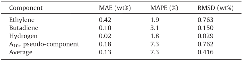
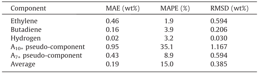
The performance of Network 3 is first evaluated separately due to the use of a different training and test set. All of the following figures use a random selection of 10% of the 1360 data points in the test set in order to maintain the legibility of the figures. The statistical metrics are calculated on the full test set. Fig. 14 illustrates the network performance on four selected output components—ethylene, 1,3-butadiene, hydrogen, and A₁₀₊ pseudocomponent. Parity plots for all other components can be found in Fig. S18, which shows that the network performance for two other major cracking products—methane and propene—is very similar to that for ethylene, which is shown in Fig. 14(a). The network performs well on the entire range of mass fractions. For ethylene, butadiene, and hydrogen, the mass fraction range is limited to about one order of magnitude. For the A₁₀₊ pseudo-component, however, the mass fractions of the dataset are spread out over nearly four orders of magnitude. By accurately predicting the mass fractions of the A₁₀₊ pseudo-component across several orders of magnitude, the network demonstrates its predictive power. Table 6 shows the statistics for these four components specifically, along with the averages for all components. In general, the network achieves an accuracy of 0.1 wt%, which is very high, given the minimal computational cost of the predictions. The entire test set of 1360 reactions is predicted in 1.716 s, or just 1.2 ms per prediction, once again on a standard Intel i7 laptop CPU. The state-of-the-art tool COILSIM1D requires several seconds to determine the detailed effluent composition for a single naphtha, indicating a tremendous speed-up for the DL ANN model. The (nearly) negligible computation times would allow such a network to be used in a larger RTO algorithm that is able to provide feedback to the process at a much higher frequency than current RTO algorithms. At this computation speed, even feed-forward process control applications are possible. The major benefit of this tremendous speed-up is, however, the ability to continuously monitor difficult-to-access process parameters with limited input, which facilitates the anticipation of sudden changes that might have a major (safety) impact on downstream operations.

In Section 2.2.2, it was mentioned that the exact reactor configuration is of secondary importance. Van Geem et al. [31] have proven that the composition of the reactor effluent for a given naphtha is defined by two severity indices accounting for outlet pressure and temperature, independently of the reactor geometry. Network 3 uses these severity indices—P/E and E/E—as input. Hence, the performance of the network will be relatively independent of the reactor geometry and can therefore be used to obtain good predictions for any type of reactor. These findings are graphically supported by Fig. S19.

《Fig. 14》

Fig. 14. Parity plots for the predictions by Network 3 on four selected components: (a) ethylene (C₂H₄); (b) butadiene; (c) hydrogen; and (d) A₁₀₊ pseudo-component. 136 of the 1360 test set data points are displayed.

《4.3. Combined effluent prediction performance》

4.3. Combined effluent prediction performance

Finally, the performance of the combination of feedstock reconstruction from easily and rapidly accessible indices and detailed effluent prediction is evaluated. This corresponds to evaluating the performance of the framework elucidated in Fig. 3.

The computational cost to run the combined framework is still very low. The 1587 test cases are simulated in just under 3.25 s–2 ms per reactor simulation, which is only a minimal increase compared with the time required to simulate the effluent from the detailed naphtha characterization. This indicates that the combined framework is at least computationally suited for integration in RTO algorithms, or even in direct process control.

Upon comparing Fig. 14 to Fig. S20 and Table 6 to Table 7, a drop in performance for the combination of Networks 1, 2, and 3 is observed. For several components, such as ethylene, butadiene, and hydrogen, the network accuracy is still very high and is close to the accuracy using the true naphtha composition. The network does have significant trouble correctly predicting the distribution between A_7–9and A₁₀₊. The parity plot for the former can be found in Fig. S21; that of the latter is provided in Fig. S20(d). The concentration of the lighter aromatics is consistently overestimated, while that of the heavier aromatics is consistently underestimated. When these two pseudo-components are further lumped into a single A₇₊ component, the network achieves an accuracy similar to the others, as shown in the next-to-last row of Table 7. A potential cause for this deviation could be a very slight, systematic underestimation of the aromatics at higher concentrations in the feedstock reconstruction. It is observed that a small variation in the aromatics content of the feedstock can significantly impact the formation of heavier aromatic compounds during the cracking process. This shows the importance of very accurate experimental data, as small measurement errors can significantly impact the results.

《Table 6》

Table 6 Statistics on the performance of Network 3 on selected components, on the test set.

《Table 7》

Table 7 Statistics on the combined performance of Networks 1, 2, and 3, on selected components, on the test set.

The clustering of the results in the parity plots of Figs. S20 and S21 is the result of the grid-like variation in the input. While the process conditions will influence the exact characteristics of the output, the naphtha composition is the main influence on the effluent composition. As only 32 different naphthas were considered for this dataset, it is not surprising that only certain regions of the effluent space are covered.

《5. Conclusions and outlook》

5. Conclusions and outlook

A framework of four interacting DL ANNs has been developed for the prediction of naphtha properties and detailed steam cracker effluent compositions, based on a limited number of commercial, or easily accessible, naphtha characteristics and process descriptors. Each of the individual networks achieves excellent performance that rivals or outperforms the accuracy of typical online analysis equipment and commercially available tools such as COILSIM1D. Using two DL ANNs to reconstruct a detailed feedstock composition from the PIONA characterization of the naphtha and its density and vapor pressure, an average MAE of 0.36 wt% across 28 different (pseudo-)components is achieved. The effluent composition can be predicted with an average MAE of 0.13 wt% when using the true, detailed naphtha composition and an average MAE of 0.19 wt% when using a naphtha composition reconstructed from the above-mentioned indices. This high predictive accuracy, combined with very low computational costs—execution of the full framework takes place in the order of milliseconds—makes the developed networks very well suited for real-time monitoring of difficult-to-access process parameters. They are also suited for use in new RTO algorithms with a much higher frequency of process adjustments than current ones. At computational delays in the order of milliseconds, even application in feed-forward process control can be considered. While the presented networks have been trained on simulations for a specific configuration of the reactor and furnace, the inclusion of reactor-independent severity indices in the input makes the network itself reactorindependent. As a result, the presented method is applicable to any type of reactor without loss of performance. The main disadvantage of DL ANNs is that the physical and interpretable meaning of the problem is lost. For detailed cause-and-effect analyses on the complex chemical mechanisms behind the process and process design, detailed kinetic models are still essential. The fact that the presented models have been trained on simulated data further advocates the development of fundamental models. However, for many practical applications, such as the above-mentioned RTO and process control, the combination of execution speed, accuracy, and ease of use are the main concerns. Due to the flexibility and predictive power of DL ANNs, several other aspects of the steam cracking process that influence the plant optimization—such as coke formation—could be approached in a similar way in the future.

《Acknowledgements》

Acknowledgements

Pieter P. Plehiers acknowledges financial support from a doctoral fellowship from the Research Foundation-Flanders (FWO). Ismaël Amghizar acknowledges financial support from SABIC Geleen. The authors acknowledge funding from the COST Action CM1404 ‘‘Chemistry of smart energy and technologies.” This work was funded by the EFRO Interreg V Flanders-Netherlands program under the IMPROVED project.

The authors also acknowledge financial support from the Long Term Structural Methusalem Funding by the Flemish Government (BOF09/01M00409).

Compliance with ethics guidelines

Pieter P. Plehiers, Steffen H. Symoens, Ismaël Amghizar, Guy B. Marin, Christian V. Stevens, and Kevin M. Van Geem declare that they have no conflict of interest or financial conflicts to disclose.

《Nomenclature》

Nomenclature

Abbreviations

2D-GC two-dimensional gas chromatography

AI artificial intelligence

ANN artificial neural network (1 hidden layer)

BP boiling point (K)

BP50 mid boiling point (K)

COP coil outlet pressure (bar, 1bar = 10⁵ Pa)

COT coil outlet temperature (K)

CPD cyclopentadiene

CPU central processing unit

DL deep learning (> 1 hidden layer)

E/E ethylene/ethane ratio

FBP final boiling point (K)

GC × GC two-dimensional gas chromatography

GPU graphics processing unit

IBP initial boiling point (K)

M/P methane/propylene ratio

MAE mean absolute error

MAPE mean absolute percentage error

MBP modeled boiling point (K)

MD mahalanobis distance

MLR multiple linear regression

MSE maximization of the Shannon entropy

P/E propylene/ethylene ratio

PC(A) principal component (analysis)

PIONA paraffins, iso-paraffins, olefins, naphthenes, aromatics

ReLU rectified linear unit

RF random forest

(R)MSD (root) mean square deviation

RTO real-time optimization

SVR support vector regression

Variables

A matrix of eigenvectors

A_k aromatics with k carbon atoms

b perceptron/layer bias

C_k hydrocarbons with k carbon atoms

d (chosen) dimensionality of the PC space

f activation function

F_a,p,n F-statistic with confidence level , p degrees of freedom, and n samples

i perceptron/layer input

i perceptron/layer input vector

I_k iso-paraffins with k carbon atoms

n number of data points in dataset

Nk naphthenes with k carbon atoms

o layer output

o perceptron output

O_k olefins with k carbon atoms

P_k paraffins with k carbon atoms

S variance-covariance matrix of the dataset

w weight

W weight matrix for single layer

w weight vector for single perceptron

x model input

x model input vector

y model output

y model output vector

z input representation in the PC space

α probability level

diagonal matrix of eigenvalues

eigenvalue

eigenvector matrix in the reduced-dimension PC space

《Appendix A. Supplementary data》

Appendix A. Supplementary data

Supplementary data to this article can be found online at https://doi.org/10.1016/j.eng.2019.02.013.

Show More