《1. Introduction》

1. Introduction

Generative adversarial networks (GANs) have emerged as one of the dominant approaches for unconditional image generation. When trained on several datasets, GANs are able to produce realistic and visually appealing samples. GAN methods train an unconditional generator that regresses real images from random noises and a discriminator that measures the difference between the generated samples and real images. GANs have received various improvements. One breakthrough was achieved by combing optimal transportation (OT) theory with GANs, such as the Wasserstein GAN (WGAN) [1]. In the WGAN framework, the generator computes the OT map from the white noise to the data distribution, and the discriminator computes the Wasserstein distance between the generated data distribution and the real data distribution.

《1.1. Manifold distribution hypothesis》

1.1. Manifold distribution hypothesis

The great success of GANs can be explained by the fact that GANs effectively discover the intrinsic structures of real datasets, which can be formulated as the manifold distribution hypothesis: A specific class of natural data is concentrated on a low-dimensional manifold embedded in the high-dimensional background space [2].

Fig. 1 shows the manifold structure of the MNIST database. Each handwritten digit image has the dimensions 28 × 28, and is treated as a point in the image space . The MNIST database is concentrated close to a low-dimensional manifold. By using the t-SNE manifold embedding algorithm [3], the MNIST database is mapped onto a planar domain, and each image is mapped onto a single point. The images representing the same digit are mapped onto one cluster, and 10 clusters are color encoded. This demonstrates that the MNIST database is distributed close to a two-dimensional (2D) surface embedded in the unit cube in .

《Fig. 1》

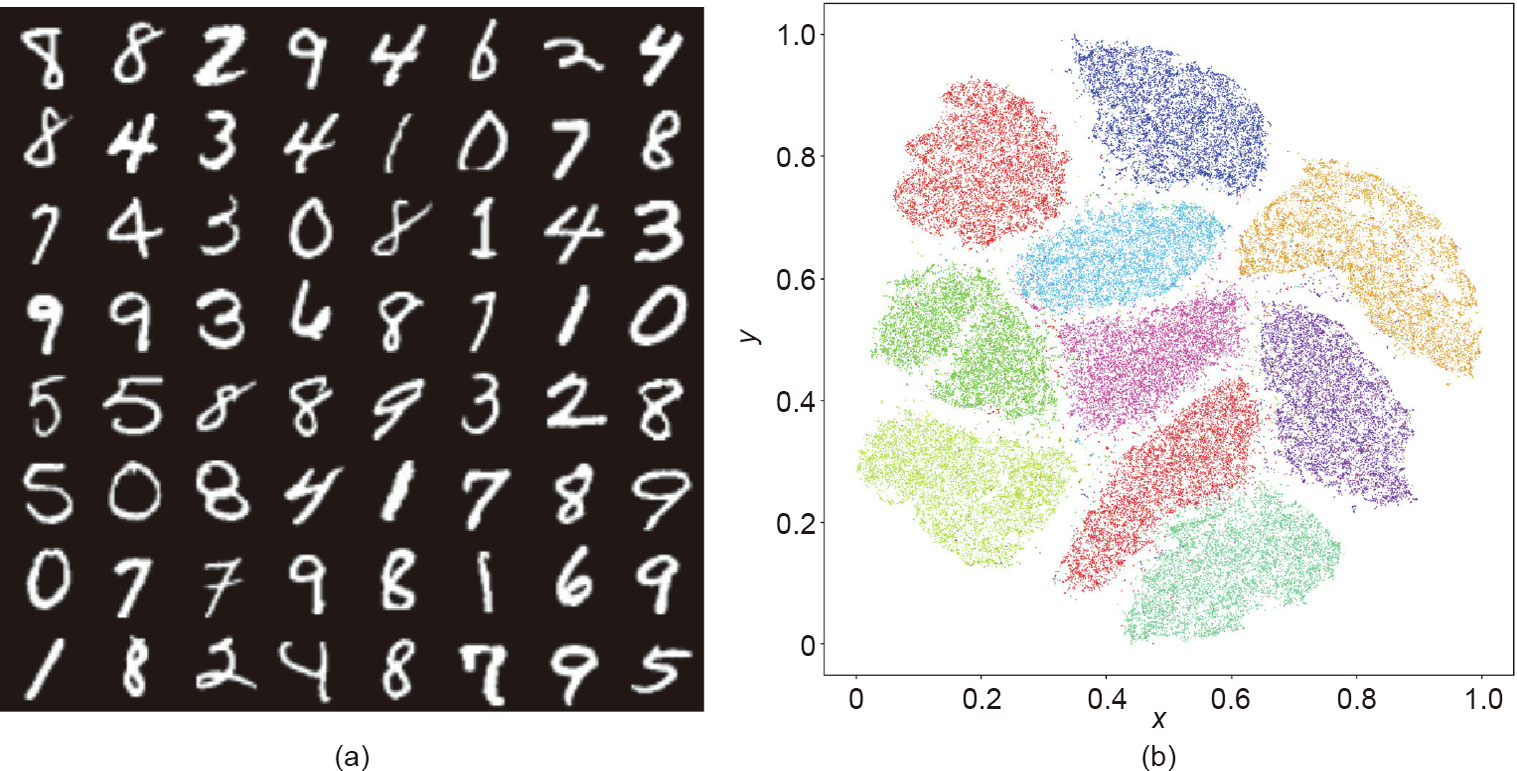
Fig. 1. Manifold distribution of the MNIST database. (a) Some handwritten digitals in MNIST database; (b) the embedded result of the digitals in two-dimensional (2D) plane by t-SNE algorithm. The x and y relative coordinates are normalized.

《1.2. Theoretic model of GANs》

1.2. Theoretic model of GANs

Fig. 2 illustrates the theoretic model of GANs. The real data distribution v is concentrated on a manifold embedded in the ambient space together show the intrinsic structure of the real datasets. A GAN model computes a generator map from the latent space Z to the manifold , where θ represents the parameter of a deep neural network (DNN). ζ  is a Gaussian distribution in the latent space, and pushes forward ζ to . The discriminator calculates a distance between the real data distribution v and the generated distribution , such as the Wasserstein distance , which is equivalent to the Kontarovich’s potential (ξ : the parameter of the discriminator).

《Fig. 2》

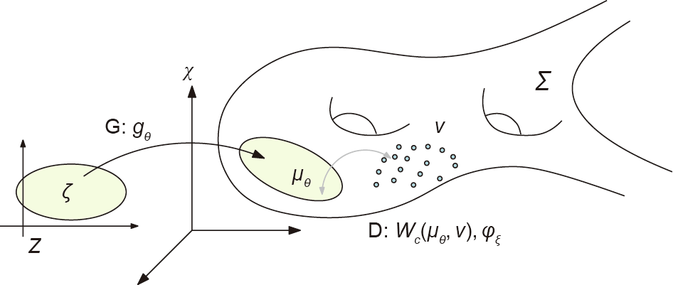
Fig. 2. The theoretic model of GANs. G: generator; D: discriminator.

Despite GANs’ advantages, they have critical drawbacks. In theory, the understanding of the fundamental principles of deep learning remains primitive. In practice, the training of GANs is tricky and sensitive to hyperparameters; GANs suffer from mode collapsing. Recently, Mescheder et al. [4] studied nine different GAN models and variants showing that gradient-descent-based GAN optimization is not always locally convergent.

According to the manifold distribution hypothesis, a natural dataset can be represented as a probability distribution on a manifold. Therefore, GANs mainly accomplish two tasks: ① manifold learning—namely, computing the decoding/encoding maps between the latent space and the ambient space; and ② probability distribution transformation, either in the latent or image space, which involves transformation between the given white noise and the data distribution.

Fig. 3 shows the decomposition of the generator map = , where h : Z → is the decoding map from the latent space to the data manifold in the ambient space, the probability distribution transformation map T: Z → Z . The decoding map h is for manifold learning, and the map T is for measure transportation.

《Fig. 3》

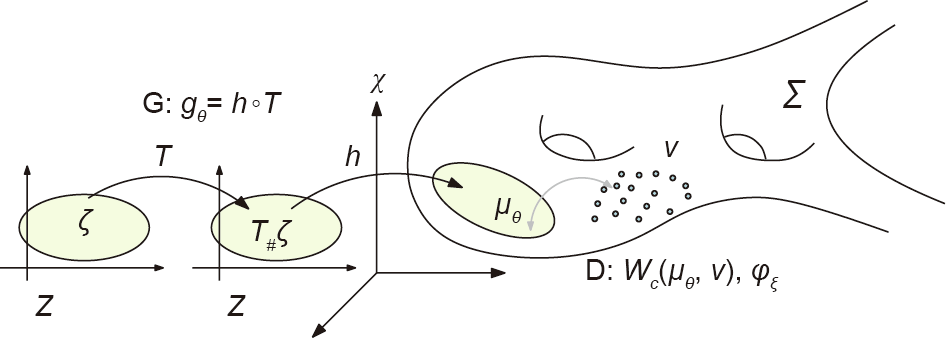
Fig. 3. The generator map is decomposed into a decoding map h and a transportation map T. T#ζ is the push-forward measure induced by T.

《1.3. Optimal transportation view》

1.3. Optimal transportation view

OT theory [5] studies the problem of transforming one probability distribution into another distribution in the most economical way. OT provides rigorous and powerful ways to compute the optimal mapping to transform one probability distribution into another distribution, and to determine the distance between them [6].

As mentioned before, GANs accomplish two major tasks: manifold learning and probability distribution transformation. The latter task can be fully carried out by OT methods directly. In detail, in Fig. 3, the probability distribution transformation map T can be computed using OT theory. The discriminator computes the Wasserstein distance between the generated data distribution and the real data distribution, which can be calculated directly using the OT method.

From the theoretical point of view, the OT interpretation of GANs makes part of the black box transparent, the probability distribution transformation is reduced to a convex optimization process using OT theory, the existence and uniqueness of the solution have theoretical guarantees, and the convergence rate and approximation accuracy are fully analyzed.

The OT interpretation also explains the fundamental reason for mode collapse. According to the regularity theory of the Monge– Ampère equation, the transportation map is discontinuous on some singular sets. However, DNN can only model continuous functions/mappings. Therefore, the target transportation mapping is outside of the functional space representable by GANs. This intrinsic conflict makes mode collapses unavoidable.

The OT interpretation also reveals a more complicated relation between the generator and the discriminator. In the current GAN models, the generator and the discriminator compete with each other without sharing the intermediate computational results. The OT theory shows that under the L² cost function, the optimal solution of the generator and the optimal solution of the discriminator can be expressed by each other in a closed form. Therefore, the competition between the generator and the discriminator should be replaced by collaboration, and the intermediate computation results should be shared to improve the efficiency.

《1.4. Autoencoder–optimal transportation model》

1.4. Autoencoder–optimal transportation model

In order to reduce the training difficulty of GANs and, in particular, to avoid mode collapses, we propose a simpler generative model based on OT theory: an autoencoder (AE)–OT model, as shown in Fig. 4.

《Fig. 4》

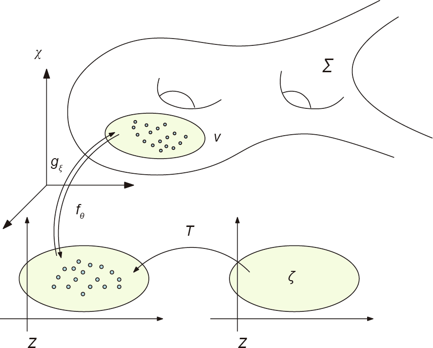
Fig. 4. A generative model, the AE–OT model, combining an AE and an OT map.

As mentioned before, the two major tasks for generative models are manifold learning and probability distribution transformation. The AE computes the encoding map,:Z → , and the decoding map : → Z, for the purpose of manifold learning. The OT map, T : Z → Z, transforms the white noise ζ to the data distribution push-forwarded by the encoding map, 

The AE–OT model has many merits. From a theoretical standpoint, the OT theory has been well established and is fully understood. By decoupling the decoding map and the OT map, it is possible to improve the theoretical rigor of generative models and make part of the black box transparent. In practice, the OT map is reduced to a convex optimization problem, the existence and the uniqueness of the solution are guaranteed, and the training process will not be trapped in the local optimum. The convex energy associated with the OT map has an explicit Hessian matrix; hence, the optimization can be performed using Newton’s method with second-order convergence, or using quasi-Newton’s method with superlinear convergence. In contrast, current generative models are based on the gradient descent method with linear convergence; the number of unknowns is equal to that of the training samples, in order to avoid the over-paramerization problem; the error bound of the OT map can be fully controlled by the sampling density in the Monte Carlo method; the hierarchical algorithm with self-adaptivity further improves the efficiency; and the parallel OT map algorithm can be implemented using a graphics processing unit (GPU). Most importantly, the AE–OT model can eliminate mode collapse.

《1.5. Contributions》

1.5. Contributions

This work interprets the GAN model using OT theory. GANs can accomplish two major tasks: manifold learning and probability distribution transformation. The latter task can be carried out using OT methods. The generator computes an OT map, and the discriminator calculates the Wasserstein distance between the generated data distribution and the real data distribution. Using Brenier’s theory, the competition between the generator and the discriminator can be replaced by collaboration; according to the regularity theory of the Monge–Ampère equation, the discontinuity of the transportation map causes mode collapse. We further propose to decouple manifold learning and probability distribution transformation by means of an AE–OT model, which makes part of the black box transparent, improves the training efficiency, and prevents mode collapse. The experimental results demonstrate the efficiency and efficacy of our method.

This paper is organized as follows: Section 2 briefly reviews the most related works in OT and GANs; Section 3 briefly introduces the fundamental theories in OT and the regularity theory of the Monge–Ampère equation; Section 4 introduces a variational framework for computing OT, which is suitable for a deep learning setting; Section 5 analyzes the GAN model from the OT perspective, explains the collaborative (instead of competitive) relation between the generator and the discriminator, and reveals the intrinsic reason for mode collapse; Section 6 reports the experimental results; and the paper concludes in Section 7.

《2. Previous works》

2. Previous works

《2.1. Optimal transportation》

2.1. Optimal transportation

The OT problem plays an important role in various kinds of fields. For detailed overviews, we refer readers to Refs. [7] and [8].

When both the input and output domains are Dirac masses, the OT problem can be treated as a standard linear programming (LP) task. In order to extend the problem to a large dataset, the authors of Ref. [9] added an entropic regularizer into the original LP problem; as a result, the regularized problem could be quickly computed with the Sinkhorn algorithm. Solomon et al. [10] then improved the computational efficiency by the introduction of fast convolution.

The second type of method for solving the OT problem computes the OT map between continuous and point-wise measures by minimizing a convex energy [6] through the connection between the OT problem and convex geometry. In Ref. [11], the authors then linked the convex-geometry-viewed OT to the Kantorovich duality by means of the Legendre dual theory. The proposed method is an extension of this method in high dimension. If both the input and output are continuous densities, solving the OT problem is equivalent to solving the famous Monge–Ampère equation, which is a highly nonlinear elliptic partial differential equation (PDE). With an additional virtual time dimension, this problem can be relaxed through computational fluid dynamics [12–14].

《2.2. Generative models》

2.2. Generative models

In the machine learning field, generative models, which are capable of generating complex and high-dimensional data, are recently becoming increasingly important and popular. To be specific, generative models are largely utilized to generate new images from given image datasets. Several methods, including deep belief networks [15] and deep Boltzmann machines [16], have been introduced in early stages. However, the training in these methods is generally tricky and inefficient. Later, a huge breakthrough was achieved from the scheme of variational AEs (VAEs) [17], where the decoders approximate real data distributions from a Gaussian distribution using a variational approach [17,18]. Various recent works following this scheme have been proposed, including adversarial AEs (AAEs) [19] and Wasserstein AEs (WAEs) [20]. Although VAEs are relatively simple to train, the images they generate look blurry. To some extent, this is because the explicitly expressed density functions may fail to represent the complexity of a real data distribution and learn the high-dimensional data distribution [21,22]. Other non-adversarial training models have been proposed, including PixelCNN [23], PixelRNN [24], and WaveNet [25]. However, due to their auto-regressive nature, the generation of new samples cannot be paralleled.

《2.3. Adversarial generative models》

2.3. Adversarial generative models

GANs [26] were proposed to solve the disadvantages of the above models. Although they are a powerful tool for generating realistic-looking samples, GANs can be difficult to train and suffer from mode collapsing. Various improvements have been proposed for better GAN training, including changing the loss function (e.g., the WGAN [1]) and regularizing the discriminators to be Lipschitz by clipping [1], gradient regularization [4,27], or spectral normalization [28]. However, the training of GANs is still tricky and requires careful hyperparameter selection.

《2.4. Evaluation of generative models》

2.4. Evaluation of generative models

The evaluation of generative models remains challenging. Early works include probabilistic criteria [29]. However, recent generative models (particularly GANs) are not amenable to such evaluation. Traditionally, the evaluation of GANs relies on visual inspection of a handful of examples or a user study. Recently, several quantitative evaluation criteria were proposed. The inception score (IS) [30] measures both diversity and image quality. However, it is not a distance metric. To overcome the shortcomings of the IS, the Fréchet inception distance (FID) was introduced in Ref. [31]. The FID has been shown to be robust to image corruption, and correlates well with visual fidelity. In a more recent work [32], precision and recall for distributions (PRD) was introduced to measure both precision and recall between generated data distribution and real data distribution. In order to fairly compare the GANs, a large-scale comparison was performed in Ref. [33], where seven different GANs and VAEs were compared under a uniform network architecture, and a common baseline for evaluation was established.

《2.5. Non-adversarial models》

2.5. Non-adversarial models

Various non-adversarial models have also been proposed recently. Generative latent optimization (GLO) [34] employs an ‘‘encoder-less AE” approach in which a generative model is trained with a non-adversarial loss function, achieving better results than VAEs. Implicit maximum likelihood estimation (IMLE) [35] proposed an iterative closest points (ICP)-related generative model training approach. Later, Hoshen and Malik [36] proposed generative latent nearest neighbors (GLANN), which combines the advantages of GLO and GLANN, in which an embedding from the image space to latent space was first found using GLO, and then a transformation between an arbitrary distribution and latent code was computed using IMLE.

Other methods directly approximate the distribution transformation map from the noise space to the image space by means of DNNs with a controllable Jacobian matrix [37–39]. Recently, the energy-based models [40–42] have been chosen to model the image distribution through the Gibbs distribution by representing the energy function with DNNs. These methods alternatively generate fake samples using the current models, and then optimize the model parameters with the generated fake samples and real samples.

《3. Optimal transportation theory》

3. Optimal transportation theory

In this section, we introduce basic concepts and theorems in classic OT theory, with a focus on Brenier’s approach and their generalization to the discrete setting. Details can be found in Villani’s book [5].

《3.1. Monge’s problem》

3.1. Monge’s problem

Suppose  are two subsets of d-dimensional Euclidean space , and μ and v are two probability measures defined on X and Y, respectively, with the following density functions:

Suppose the total measures are equal,  ;  that is

We only consider maps that preserve the measures.

Definition 3.1 (measure-preserving map). A map T: X → Y is measure preserving if for any measurable set B Y, the set T ^-1 (B) is μ-measurable and , that is,

The measure-preserving condition is denoted as = v , where  is the push-forward measure induced by T.

Given a cost function  , which indicates the cost of moving each unit mass from the source to the target, the total transport cost (C_t ) of the map  T : X → Y is defined to be

Monge’s problem of OT arises from finding the measure- preserving map that minimizes the total transport cost.

Problem 3.2 (Monge’s [43]; MP). Given a transport cost function  , find the measure-preserving map  T : X → Y that minimizes the total transport cost:

Definition 3.3 (OT map). The solutions to Monge’s problem are called the OT maps. The total transportation cost of an OT map is called the Wasserstein distance between μ and v , denoted as .

《3.2. Kontarovich’s approach》

3.2. Kontarovich’s approach

Depending on the cost function and measures, an OT map between (X, μ ) and (Y, v ) may not exist. Kontarovich relaxed the transportation maps to transportation plans, and defined the joint probability measure , such that the marginal probability of ρ is equal to μ and v , respectively. Let the projection maps formally be , then define the joint measure class as follows:

Problem 3.4 (Kontarovich’s; KP). Given a transport cost function ,  find the joint probability measure :   that minimizes the total transport cost.

KP can be solved using the LP method. Due to the duality of LP, Eq. (7) (the KP equation) can be reformulated as the duality problem (DP) as follows:

Problem 3.5 (duality; DP). Given a transport cost function  , find the real functions   and  , such that

The maximum value of Eq. (8) gives the Wasserstein distance. Most existing WGAN models are based on the duality formulation under the L¹ cost function.

Definition 3.6 (c-transformation). The c-transformation of  is defined as :

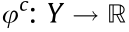The DP can then be rewritten as follows:

《3.3. Brenier’s approach》

3.3. Brenier’s approach

For the quadratic Euclidean distance cost, the existence, uniqueness, and intrinsic structure of the OT map were proven by Brenier [44].

Theorem 3.7 (Brenier’s [44]). Suppose X and Y are subsets of the Euclidean space  and the transportation cost is the quadratic Euclidean distance  .  Furthermore, μ is absolutely continuous and μ and v have finite second-order moments

then there exists a convex function , the so-called Brenier’s potential, whose gradient map   gives the solution to MP:

The Brenier’s potential is unique up to a constant; hence, the optimal mass transportation map is unique.

Assuming that the Briener potential is C ² smooth, then it is the solution to the following Monge–Ampère equation:

For the L² transportation cost  in , the c-transform and the classical Legendre transform have special relations.

Definition 3.8 (Legendre transform). Given a function , its Legendre transform is defined as follows:

It can be shown that the following relation holds when

Theorem 3.9 (Brenier’s polar factorization [44]). Suppose X and Y are the Euclidean space , μ is absolutely continuous with respect to the Lebesgue measure, and a mapping  pushes μ forward to v , = v, then there exists a convex function , such that , where   is measure preserving, =μ. Furthermore, this factorization is unique.

The following theorem is well known in OT theory:

Theorem 3.10 (Villani [5]). Given μ and v on a compact convex domain  ,  there exists an OT plan ρ for the cost =, with h strictly convex. It is unique and of the form (id, T_# ) μ (id: identity map), provided that l is absolutely continuous and  is negligible. Moreover, there exists a Kantorovich’s potential φ, and T can be represented as follows:

In this case, the Brenier’s potential u and the Kantorovich’s potential φ are related by the following:

《3.4. Regularity of OT maps》

3.4. Regularity of OT maps

Let and be two bounded smooth open sets in , and let  be two probability measures on such that =0  and =0. Assume that f and g are bounded away from zero and infinity on and , respectively.

3.4.1. Convex target domain

Definition 3.11 (Hölder continuous). A real or complex-valued function f on a d-dimensional Euclidean space satisfies a Hölder condition, or is Hölder continuous, when there are nonnegative real constants C , α  > 0, such that  for all x and y in the domain of f.

Definition 3.12 (Hölder space). The Hölder space , where  is an open subset of some Euclidean space and k ≥0 is an integer, consists of those functions on having continuous derivatives up to order k and such that the kth partial derivatives are Hölder continuous with exponent α , where 0 <α ≤1.   means the above conditions hold on any compact subset of .

Theorem 3.13 (Caffarelli [45]). If is convex, then the Brenier’s potential u is strictly convex; furthermore,

(1) If    for some λ > 0, then u  .

(2) If  and , with  f, g > 0, then u  and  k ≥ 0, α （0,1）.

3.4.2. Non-convex target domain

If is not convex and there exist f and g that are smooth such that  , then the OT map  is discontinuous at singularities.

Definition 3.14 (subgradient). Given an open set  and a convex function u :  , for  , the subgradient (subdifferential) of u at x is defined as follows:

It is obvious that u (x ) is a closed convex set. Geometrically, if ,  then the hyperplane   touches u from below at x ; that is,  in Ω and  ,  where  is a supporting plane to u at x .

The Brenier’s potential u is differentiable at x if its subgradient   is a singleton. We classify the points according to the dimensions of their subgradients, and define the sets ,  

It is obvious that  is the set of regular points, and , where k > 0, is the set of singular points. We also define the reachable subgradients at x as follows:

It is well known that the subgradient is equal to the convex hull of the reachable subgradient:

Theorem 3.15 (regularity). Let  be two bounded open sets, let f, g :  be two probability densities that are zero outside  and , and are bounded away from zero and infinity on  and ,  respectively. Denote by T =→ the OT map provided by Theorem 3.7. Then there exist two relatively closed sets   and  with =0 such that T : is a homeomorphism of class  for some α > 0.

We call  the singular set of the OT map →.  Fig. 5 illustrates the singularity set structure, computed using the algorithm based on Theorem 4.2. We obtain the following:

《Fig. 5》

Fig. 5. Singularity structure of an OT map.

The subgradient of ,  is the entire inner hole of , while  is the shaded triangle. For each point on  is a line segment outside .  is the bifurcation point of  and  The Brenier’s potential on  is not differentiable, and the OT map   on them is discontinuous.

《4. Computational algorithm》

4. Computational algorithm

Brenier’s theorem can be directly generalized to the discrete situation. In GAN models, the source measure μ is given as a uniform (or Gaussian) distribution defined on a compact convex domain ; the target measure v is represented as the empirical measure, which is the sum of the Dirac measures:

where Y =  are training samples, with the weights  is the characteristic function.

Each training sample corresponds to a supporting plane of the Brenier’s potential, denoted as follows:

where the height is an unknown variable. We represent all the height variables as .

An envelope of a family of hyper-planes in the Euclidean space is a hypersurface that is tangential to each member of the family at some point, and these points of tangency together form the whole envelope. As shown in Fig. 6, the Brenier’s potential    is a piecewise linear convex function determined by h, which is the upper envelope of all its supporting planes:

The graph of the Brenier’s potential is a convex polytope. Each supporting plane  corresponds to a facet of the polytope. The projection of the polytope induces a cell decomposition of , where each supporting plane  projects onto a cell  is
any point in :

The cell decomposition is a power diagram. The μ -measure of   is denoted as :

The gradient map  maps each cell  to a single point :

Given the target measure v in Eq. (17), there exists a discrete Brenier’s potential in Eq. (19) whose projected μ volume of each facet   is equal to the given target measure  This was proved by Alexandrov [46] in convex geometry.

Theorem 4.1 (Alexandrov [46]). Suppose is a compact convex polytope with a non-empty interior in  are distinct k unit vectors, the (n + 1)th coordinates are negative, and v₁ , ..., v_k > 0 so that . Then there exists a convex polytope  with the exact k codimension-1 faces F₁ , ..., F_k so that  is the normal vector to F_i and the intersection between  and the projection of F_i has the volume v_i . Furthermore, such P is unique up to vertical translation.

《Fig. 6》

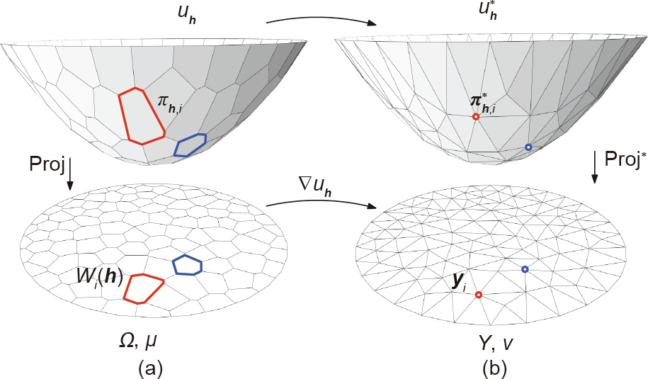
Fig. 6. (a) Piecewise linear Brenier’s potential (u_h ) and (b) its Legendre transformation :the Legendre dual of  :the gradient of u_h ; Proj: project map;  Proj^*: the projection map in the Legendre dual space.

Alexandrov’s proof for the existence of the solution is based on algebraic topology, which is not constructive. Recently, Gu et al. [6] provided a constructive proof based on the variational approach.

Theorem 4.2 (Ref. [6]). Let μ be a probability measure defined on a compact convex domain  in  ,  and let Y = be a set of distinct points in . Then for any v₁ , v₂ , ..., v_n > 0 with , there exists  ,  which is unique up to adding a constant (c, c, ..., c ), so that  , for all i. The vector h is the unique minimum argument of the following convex energy:

defined on an open convex set

Furthermore,  minimizes the quadratic cost

among all transport maps .

The gradient of the above convex energy in Eq. (23) is given by the following:

The i th row and jth column element of the Hessian of the energy is given by the following:

As shown in Fig. 6, the Hessian matrix has an explicit geometric interpretation. Fig. 6(a) shows the discrete Brenier’s potential u_h while Fig. 6(b) shows its Legendre transformation  using Definition 3.8. The Legendre transformation can be constructed geometrically: For each supporting plane , we construct the dual point  ;  the convex hull of the dual points  is the graph of the Legendre transformation .

The projection of  induces a triangulation of Y =, which is the weighted Delaunay triangulation. As shown in Fig. 7, the power diagram in Eq. (20) and the weighted Delaunay triangulation are Poincaré dual to each other: If, in the power diagram,  intersect at a (d – 1)-dimensional cell, then in the weighted Delaunay triangulation, connects with   The element of the Hessian matrix in Eq. (27) is the ratio between the μ volume of the (d – 1) cell in the power diagram and the length of the dual edge in the weighted Delaunay triangulation.

《Fig. 7》

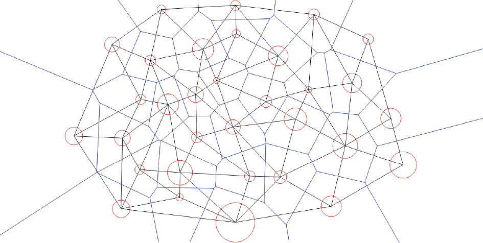
Fig. 7. Power diagram (blue) and its dual-weighted Delaunay triangulation (black).

The conventional power diagram can be closely related to the above theorem.

Definition 4.3 (power distance). Given a point  with a power weight , the power distance is given by the following:

Definition 4.4 (power diagram). Given the weighted points 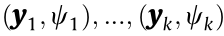,  the power diagram is the cell decomposition of :

where each cell is a convex polytope:

The weighted Delaunay triangulation, denoted as ,  is the Poincaré dual to the power diagram; if ,  then there is an edge connecting in the weighted Delaunay triangulation. Note that   is equivalent to

Let ;  then we rewrite the definition of  as follows:

In practice, our goal is to compute the discrete Brenier’s potential Eq. (19) by optimizing the convex energy Eq. (23). For lowdimensional cases, we can directly use Newton’s method by computing the gradient Eq. (26) and the Hessian matrix Eq. (27). For deep learning applications, direct computation of the Hessian matrix is unfeasible; instead, we can use the gradient descend method or quasi-Newton’s method with superlinear convergence. The key of the gradient is to estimate the μ volume . This can be done using the Monte Carlo method: We draw n random samples from the distribution μ , and count the number of samples falling within , which is the ratio converging to the μ  volume. This method is purely parallel and can be implemented using a GPU. Moreover, we can use a hierarchical method to further improve the efficiency: First, we classify the target samples to clusters, and compute the OT map to the mass centers of the clusters; second, for each cluster, we compute the OT map from the corresponding cell to the original target samples within the cluster.

In order to avoid mode collapse, we need to find the singularity sets in . As shown in Fig. 8, the target Dirac measure has two clusters; the source is the uniform distribution on the unit planar disk. The graph of the Brenier’s potential function is a convex polyhedron with a ridge in the middle. The projection of the ridge on the disk is the singularity set , and the optimal mapping is discontinuous on . In general cases, if two cells and are adjacent, then we compute the angle between the normals to the corresponding support planes:

If  is greater than a threshold, then the common facet   is in the discontinuity singular set.

《Fig. 8》

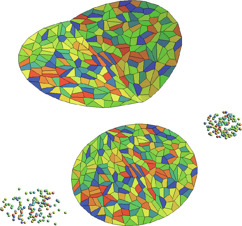
Fig. 8. Singularity set of the Brenier’s potential function and discontinuity set of the OT map.

《5. GANs and optimal transportation》

5. GANs and optimal transportation

OT theory lays down the theoretical foundation for GANs. Many recent works, such as the WGAN [1], gradient penalty WGAN (WGAN-GP) [27], and relaxed Wasserstein with applications to GAN (RW-GAN) [47], use the Wasserstein distance to measure the deviation between the generated data distribution and the real data distribution.

From the OT perspective, the optimal solutions for the generator and discriminator are related by a closed form; hence, the generator and the discriminator should collaborate instead of compete. More details can be found in Ref. [11]. Furthermore, the regularity theory of the solutions to the Monge–Ampère equation can explain the mode collapse in GANs [48].

《5.1. Competition versus collaboration》

5.1. Competition versus collaboration

The OT view of the WGAN [1] is illustrated in Fig. 2. According to the manifold distribution hypothesis, the real data distribution v is close to a manifold embedded in the ambient space . The generator computes the decoding map  from the latent space Z to the ambient space, and transforms the white noise (i.e., the Gaussian distribution) to the generated distribution, . The discriminator computes the Wasserstein distance between  and the real data distribution ,  by computing the 
Kantorovich’s potential .  Both  and are realized by DNNs.

In the training process, the generator improves in order to better approximate v by ;  the discriminator refines the Kantorovich’s potential to improve the estimation of the Wasserstein distance. The generator and the discriminator compete with each other, without sharing intermediate computational results. Under the L₁ cost function, the alternative training process of the WGAN can be formulated as the min–max optimization of expectations:

But if we change the cost function to be L² distance, then according to Theorem 3.10, at the optimum, the Brenier’s potential u and the Kontarovich’s potential φ are related by a closed form of Eq. (16), . The generator pursues the OT map  ; the discriminator computes φ. Hence, once the generator reaches the optimum, the optimal solution for the discriminator can be obtained without any training, and vice versa.

In more detail, suppose at the kth iteration, the generator map is . The discriminator computes the Kontarovich’s potential , which gives the Wasserstein distance between the current generated data distribution  and the real data distribution v ; gives the OT map from  to v . Therefore, we obtain the following:

This means that the generator map can be updated by the following:

This conclusion shows that, in principle, the training process of the generator can be skipped; in practice, the efficiency can be improved greatly by sharing the intermediate computational results. Therefore, in designing the architectures of GANs, collaboration is better than competition.

《5.2. Mode collapse and regularity》

5.2. Mode collapse and regularity

Although GANs are powerful for many applications, they have critical drawbacks: First, the training of GANs is tricky, sensitive to hyperparameters, and difficult to converge; second, GANs suffer from mode collapsing; and third, GANs may generate unrealistic samples. The difficulties of convergence, mode collapse, and the generation of unrealistic samples can be explained by the regularity Theorem 3.15 of the OT map.

According to Brenier’s polar factorization, Theorem 3.9, any measure-preserving map can be decomposed into two maps, one of which is an OT map, which is a solution to the Monge–Ampère equation. According to the regularity Theorem 3.15, if the support of the target measure v has multiple connected components— that is, if v has multiple modes, or is non-convex—then the OT map T : → is discontinuous on the singular set  .

Fig. 9 shows the multi-cluster case: has two connected components, where the OT map T is discontinuous along . Fig. 10 shows that even is connected, albeit non-convex. is a rectangle, is a dumbbell shape, the density functions are constants, the OT map is discontinuous, and the singularity set .

《Fig. 9》

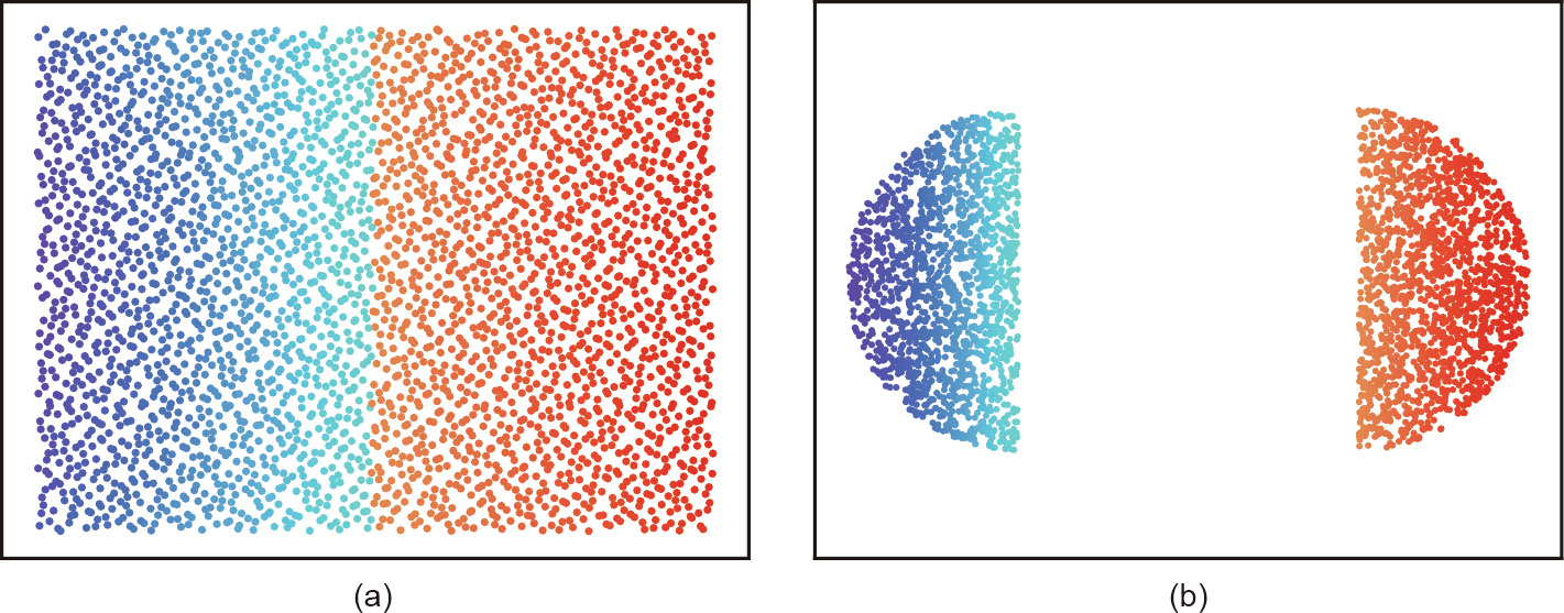
Fig. 9. Discontinuous OT map, produced by a GPU implementation of an algorithm based on Theorem 4.2: (a) is the source domain and (b) is the target domain. The middle line in (a) is the singularity set .

《Fig. 10》

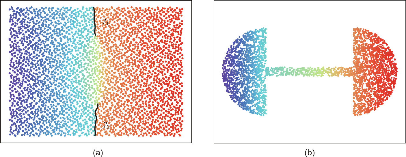
Fig. 10. Discontinuous OT map, produced by a GPU implementation of an algorithm based on Theorem 4.2: (a) is the source domain and (b) is the target domain. in (a) are two singularity sets.

Fig. 11 shows an OT map between two probability measures in .  Both the source measure μ and the target measure v are uniform distributions; the support of is the unit solid ball, and the support of is the solid Stanford bunny. We compute the Brenier’s potential u :  based on Theorem 4.2. In order to visualize the mapping, we interpolate the probability measure as follows:

Fig. 11 shows the support of the interpolated measure . The foldings on the surface are the singularity sets, where the OT map is discontinuous.

《Fig. 11》

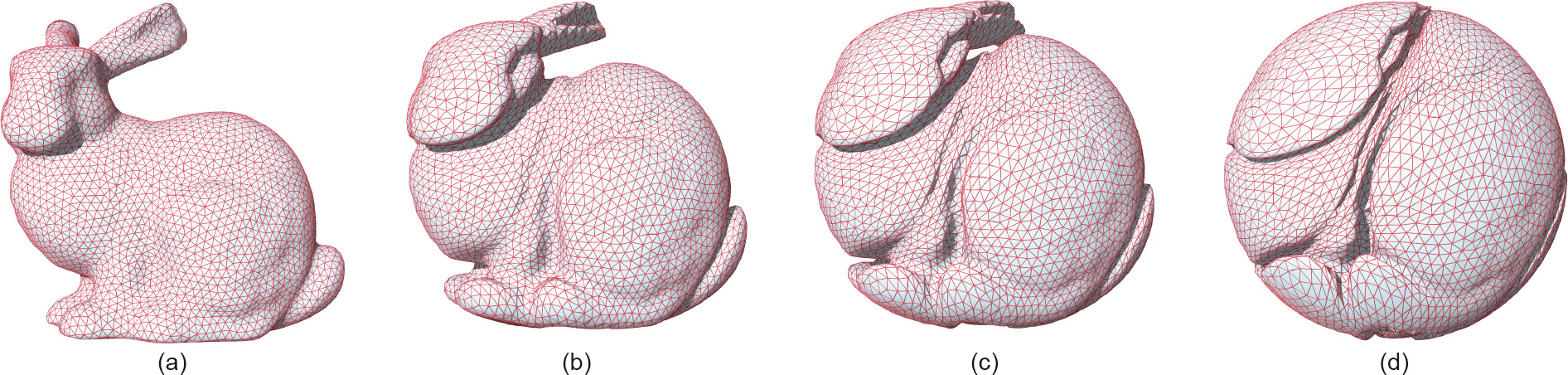
Fig. 11. OT from the Stanford bunny to a solid ball. The singular sets are the foldings on the boundary surface. (a–d) show the deformation procedure.

In a general situation, due to the complexity of the real data distributions, the embedding manifold , and the encoding/decoding maps, the supports of the target measures are rarely convex; therefore, the transportation mapping cannot be globally continuous.

On the other hand, general DNNs, such as rectified linear unit (ReLU) DNNs, can only approximate continuous mappings. The functional space represented by ReLU DNNs does not contain the desired discontinuous transportation mapping. The training process or, equivalently, the searching process will lead to three alternative situations:

(1) The training process is unstable, and does not converge.

(2) The searching converges to one of the multiple connected components of K, and the mapping converges to one continuous branch of the desired transportation mapping. This means that a mode collapse is encountered.

(3) The training process leads to a transportation map, which covers all the modes successfully, but also covers the regions outside . In practice, this will induce the phenomenon of generating unrealistic samples, as shown in the middle frame of Fig. 12.

Therefore, in theory, it is impossible to approximate OT maps directly using DNNs.

《Fig. 12》

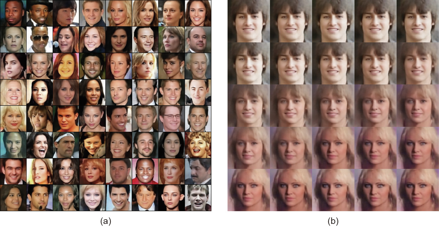
Fig. 12. Facial images generated by an AE–OT model. (a) Generated realistic facial images; (b) a path through a singularity. The image in the center of (b) shows that the transportation map is discontinuous.

《5.3. AE–OT model》

5.3. AE–OT model

As shown in Fig. 4, we separate the two main tasks of GANs: manifold learning and probability distribution transformation. The first task is carried out by an AE to compute the encoding/ decoding maps ; the second task is accomplished using the explicit variational method to compute the OT map T in the latent space. The real data distribution v is pushed forward by the encoding map , inducing .  In the latent space, T maps the uniform distribution μ to .

The AE–OT model has many advantages. In essence, finding the OT map is a convex optimization problem; the existence and the uniqueness of the solution are guaranteed. The training process is stable and has superlinear convergence by using quasiNewton’s method. The number of unknowns is equal to that of the training samples, avoiding over-paramerization. The parallel OT map algorithm can be implemented using a GPU. The error bound of the OT map can be controlled by the sampling density in the Monte Carlo method. The hierarchical algorithm with selfadaptivity further improves the efficiency. In particular, the AE– OT model can eliminate mode collapse.

《6. Experimental results》

6. Experimental results

In this section, we report our experimental results.

《6.1. Training process》

6.1. Training process

The training of the AE–OT model mainly includes two steps: training the AE and finding the OT map. The OT step is accomplished using a GPU implementation of the algorithm, as described in Section 4. In the AE step, during the training process, we adopt the Adam algorithm [49] to optimize the parameters of the neutral network, with a learning rate of 0.003, β₁ = 0.5, and β₂ = 0.999. When the L² loss stops descending, which means that the network has found a good encoding map, we freeze the encoder part and continue to train the network for the decoding map. The training loss before and after the freezing of the encoder is shown in Table 1. Next, in order to find the OT map from the given distribution (here, we use uniform distribution) to the distribution of latent features, we randomly sample 100N random points from the uniform distribution to compute the gradient of the energy. Here, N is the number of latent features of the dataset. Also, in the experiment, is set to be different for different datasets. To be specific, for the MNIST and Fashion-MNIST datasets, is set to be 0.75, while for the CIFAR-10 and CelebA datasets, it is set to be 0.68 and 0.75, respectively.

《Table 1》

Table 1 The L² loss of the AEs before and after the freezing of the encoder.

Our AE–OT model was implemented using PyTorch on a Linux platform. All the experiments were conducted on a GTX1080Ti.

《6.2. Transportation map discontinuity test》

6.2. Transportation map discontinuity test

In this experiment, we want to test our hypothesis: In most real applications, the support of the target measure is non-convex, the singularity set is non-empty, and the probability distribution map is discontinuous along the singularity set.

As shown in Fig. 12, we use an AE to compute the encoding/ decoding maps from the CelebA dataset (, v ) to the latent space Z ; the encoding map : →Z pushes forward v to  on the latent space. In the latent space, we compute the OT map based on the algorithm described in Section 4, T : Z  → Z , where T maps the uniform distribution in a unit cube ζ  to . Then we randomly draw a sample Z from the distribution ζ and use the decoding map  :Z →to map T (z ) to a generated human facial image  T (z ).  Fig. 12(a) demonstrates the realistic facial images generated by this AE–OT framework.

If the support of the push-forward measure   in the latent space is non-convex, there will be a singularity set , where k > 0. We would like to detect the existence of . We randomly draw line segments in the unit cube in the latent space, and then
densely interpolate along this line segment to generate facial images. As shown in Fig. 12(b), we find a line segment γ , and generate a morphing sequence between a boy with a pair of brown eyes and a girl with a pair of blue eyes. In the middle, we generate 
a face with one blue eye and one brown eye, which is definitely unrealistic and outside . This result means that the line segment γ goes through a singularity set . where the transportation map T is discontinuous. This also shows that our hypothesis is correct: The support of the encoded human facial image measure on the latent space is non-convex.

As a byproduct, we find that this AE–OT framework improves the training speed by a factor of five and increases the convergence stability, since the OT step is a convex optimization. Thus, it provides a promising way to improve existing GANs.

《6.3. Mode collapse comparison》

6.3. Mode collapse comparison

Since the synthetic dataset consists of explicit distributions and known modes, mode collapse can be accurately measured. We chose two synthetic datasets that have been studied or proposed in prior works [50,51]: a 2D grid dataset.

For a choice of the measurement metric of mode collapse, we adopted three previously used metrics [50,51]. Number of modes counts the quantity of modes captured by the samples produced by a generative model. In this metric, a mode is considered as lost if no sample is generated within three standard deviations of that mode. Percentage of high-quality samples measures the proportion of samples that are generated within three standard deviations of the nearest mode. The third metric, used in Ref. [51], is the reverse Kullback–Leibler (KL) divergence. In this metric, each generated sample is assigned to its nearest mode, and we count the histogram of samples assigned on each mode. This histogram then forms a discrete distribution, whose KL divergence with the histogram formed by real data is then calculated. Intuitively, this measures how well the generated samples balance among all modes regarding the real distribution.

In Ref. [51], the authors evaluated GAN [26], adversarially learned inference (ALI) [52], minibatch discriminati (MD) [30], and PacGAN [51] on synthetic datasets with the above three metrics. Each experiment was trained under the same generator architecture with a total of approximately 4 × 10⁵ training parameters. The networks were trained on 1 × 10⁵ samples for 400 epochs. For the AE–OT experiment, since the source space and target space are both 2D, there is no need to train an AE. We directly compute a semi-discrete OT that maps between the uniform distribution on the unit square and the empirical real data distribution. Theoretically, the minimum amount of real sample needed for OT to recover all modes is one sample per mode. However, this may lead to the generation of low-quality samples during the interpolation process. Therefore, for OT computation, we take 512 real samples, and new samples are generated based on this map. We note that, in this case, there are only 512 parameters to optimize in OT computing, and the optimization process is stable due to the existence of the convex positive-definite Hessian. Our results are provided in Table 2, and benchmarks of previous methods are copied from Ref. [51]. For illustration purposes, we plotted our results on synthetic datasets along with those of GAN and PacGAN in Fig. 13.

《Table 2》

Table 2 Mode collapse comparison for the 2D grid dataset.

《Fig. 13》

Fig. 13. Mode collapse comparison on a 2D grid dataset. (a) GAN; (b) PacGAN4; (c) AE–OT. Orange marks are real samples and green marks are generated ones.

《6.4. Comparison with the state of the art》

6.4. Comparison with the state of the art

We designed experiments to compare our proposed AE–OT model with state-of-the-art generative models, including the adversarial models evaluated by Lucic et al. in Ref. [33], and the non-adversarial models studied by Hoshen and Malik in Ref. [36].

For the purpose of fair comparison, we used the same testing datasets and network architecture. The datasets included MNIST [53], Fashion-MNIST [54], CIFAR-10 [55], and CelebA [56], similar to those tested in Refs. [31,36]. The network architecture was similar to that used by Lucic et al. in Ref. [33]. In particular, in our AE–OT model, the network architecture of the decoder was the same as that of the generators of GANs in Ref. [33], and the encoder was symmetric to the decoder

We compared our model with state-of-the-art generative models using the FID score [31] and PRD curve as the evaluation criteria. The FID score measures the visual fidelity of the generated results and is robust to image corruption. However, the FID score is sensitive to mode addition and dropping [33]. Hence, we also used the PRD curve, which can quantify the degree of mode dropping and mode inventing on real datasets [32].

6.4.1. Comparison with FID score

The FID score is computed as follows: ① Extract the visually meaningful features of both the generated and real images by running the inception network [30], ② fit the real and generated feature distributions with Gaussian distributions; and ③ compute the distance between the two Gaussian distributions using the following formula:

where 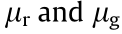 represent the means of the real and generated distributions, respectively; and  and represent the variances of these distributions.

The comparison results are summarized in Tables 3 and 4. The statistics of various GANs come from Lucic et al. [33], and those of the non-adversarial generative models come from Hoshen and Malik [36]. In general, our proposed model achieves better FID scores than the other state-of-the-art generative models.

《Table 3》

Table 3 Quantitative comparison with FID-I.

The best result is shown in bold. MM: manifold matching; NS: non-saturating; LSGAN: least squares GAN; BEGAN: boundary equilibrium GAN.

《Table 4》

Table 4 Quantitative comparison with FID-II.

The best result is shown in bold.

Theoretically, the FID scores of our AE–OT model should be close to those of the pre-trained AEs; this is also validated by our experiments.

The fixed network architecture of our AE was adopted from Lucic et al. [33]; its capacity is not large enough to encode CIFAR-10 or CelebA, so we had to down-sample these datasets. We randomly selected 2.5 × 10⁴ images from CIFAR-10 and 1 × 10⁴ images from CelebA to train our model. Even so, our model obtained the best FID score in CIFAR-10. Dut to the limited capacity of the InfoGAN model, the performance of the AE of CelebA, whose FID of 67.5 is not ideal, further caused the FID of the generated dataset to be 68.4. By adding two more convolutional layers to the AE architecture, the L² loss in CelebA was less than 0.03, and the FID score beat all other models (28.6, as shown in the bracket of Table 4).

6.4.2. Comparison with the PRD curve

The FID score is an effective method to measure the difference between the generated distribution and the real data distribution, but it mainly focuses on precision, and cannot accurately capture what portion of real data a generative model can cover. The method proposed in Ref. [32] disentangles the divergence between distributions into two components: precision and recall.

Given a reference distribution P and a learned distribution Q, the precision intuitively measures the quality of samples from Q, while the recall measures the proportion of P that is covered by Q.

We used the concept of (F₈, F_1/8) introduced by Sajjadi et al. in Ref. [32] to quantify the relative importance of precision and recall. Fig. 14 summarizes the comparison results. Each dot represents a specific model with a set of hyperparameters. The closer a dot is to the upper-right corner, the better the performance of the model is. The blue and green dots show the GANs and VAEs evaluated in Ref. [32], the khaki dot represents the GLANN model in Ref. [36], and the red dot is our AE–OT model.

《Fig. 14》

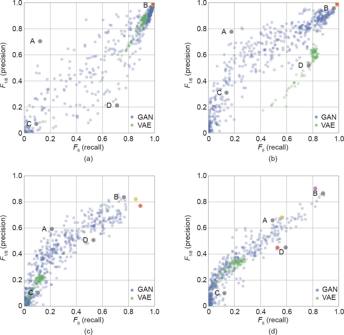
Fig. 14. A comparison of the precision–recall pair in (F₈, F_1/8) in the four datasets. (a) MNIST; (b) Fashion-MNIST; (c) CIFAR-10; (d) CelebA. The khaki dots are the results of Ref. [36]. The red dots are the results of the proposed method. The purple dot in the fourth subfigure corresponds to the results of the architecture with two more convolutional layers.

It is clear that our proposed model outperforms others for MNIST and Fashion-MNIST. For the CIFAR-10 dataset, the precision of our model is slightly lower than those of GANs and GLANN, but the recall is the highest. For the CelebA dataset, due to the limited capacity of the AE, the performance of our model is not impressive. However, after adding two more convolutional layers to the AE, our model achieves the best score.

6.4.3. Visual comparison

Fig. 15 shows a visual comparison between the images generated by our proposed method and those generated by the GANs studied by Lucic et al. in Ref. [33] and the non-adversarial models studied by Hoshen and Malik in Ref. [36]. The first column shows the original images, the second column shows the results generated by the AE, the third column shows the best generating results of the GANs in Lucic et al. [33], the fourth column displays the results generated by the models of Hoshen and Malik [36], and the fifth column displays the results from our method. It is clear that our method generates high-quality images and covers all modes.

《Fig. 15》

Fig. 15. A visual comparison of the four datasets. The first column (a) shows the real data; the second column (b) is generated by an AE; the third column (c) illustrates the generating results of the GANs [33] with the highest precision-recall scores of (F₈, F_1/8), corresponding to the B dots in Fig. 14; the fourth column (d) gives the results of Ref. [36]; and the last column (e) shows the results of the proposed method.

《7. Conclusion》

7. Conclusion

This work uses OT theory to interpret GANs. According to the data manifold distribution hypothesis, GANs mainly accomplish two tasks: manifold learning and probability distribution transformation. The latter task can be carried out using the OT method directly. This theoretical understanding explains the fundamental reason for mode collapse, and shows that the intrinsic relation between the generator and the discriminator should be collaboration instead of competition. Furthermore, we propose an AE–OT model, which improves the theoretical rigor, training stability, and efficiency, and eliminates mode collapse.

Our experiment validates our assumption that if the distribution transportation map is discontinuous, then the existence of the singularity set leads to mode collapse. Furthermore, when our proposed model is compared with the state of the art, our method eliminates the mode collapse and outperforms the other models in terms of the FID score and PRD curve.

In the future, we will explore the theoretical understanding of the manifold learning stage, and use a rigorous method to make this part of the black box transparent.

《Acknowledgements》

Acknowledgements

The project is partially supported by the National Natural Science Foundation of China (61936002, 61772105, 61432003, 61720106005, and 61772379), US National Science Foundation (NSF) CMMI-1762287 collaborative research ‘‘computational framework for designing conformal stretchable electronics, Ford URP topology optimization of cellular mesostructures’ nonlinear behaviors for crash safety,” and NSF DMS-1737812 collaborative research ‘‘ATD: theory and algorithms for discrete curvatures on network data from human mobility and monitoring.”

《Compliance with ethics guidelines》

Compliance with ethics guidelines

Na Lei, Dongsheng An, Yang Guo, Kehua Su, Shixia Liu, Zhongxuan Luo, Shing-Tung Yau, and Xianfeng Gu declare that they have no conflicts of interest or financial conflicts to disclose.