《1. Introduction》

1. Introduction

For a long time, the classical method used to analyze the security and stability of power transmission and distribution systems [1,2] is the point-wise method, i.e., the conclusion that a system is secure/unsecure or stable/unstable is drawn by simulation calculation in one or more fault modes of a specific scenario (operation mode; i.e., operation point). This method still plays an important role in power system analysis. However, it is difficult to use this method to quickly and directly obtain an overall evaluation of power system operation states, such as how far the current operation point is from the stability boundary, how large the stability margin is, and so on. How to comprehensively consider power flow constraints and various stability constraints in a series of power system optimization problems without affecting the decisionmaking speed is always a difficult issue. The computational burden of power system probabilistic security assessment is even more unimaginable.

Wu et al. [3] introduced the concept of probabilistic security assessment and Refs. [4–6] put forward the concept of steadystate security region (SSSR) and dynamic security region (DSR) in the injection space. Security region (SR) methodology is a new methodology developed on the basis of the point-wise method. It addresses problems from the perspective of region and describes a region in which a power system can operate securely as a whole (the green area in Fig. 1 [7] is the SR). The relative relation between system operation points and SR boundary can provide information on the security margin and optimal control direction, which will enable power system operators to perform online real-time security monitoring, assessment, and control in a more scientific and efficient manner. The SRs introduced in this paper are mainly defined in the power injection space (or decision space). They are uniquely determined for a given network topology and given system component parameters (as well as location and clearing process of faults for DSR), and do not vary with operation states. Therefore, it is only necessary to calculate the SR boundaries (i.e., hyperplane (HP) coefficients, etc.) once and store them in a database for use in future analysis and calculation, without adding calculation burden to online application. In view of this advantage, this paper only introduces the SRs that are irrelevant to the operation states and does not cover the method of determining SR boundaries based on operation states obtained through real-time measurement.

《Fig. 1》

Fig. 1. Schematic diagram of a SR [7].

The mathematical description [3] of power system security and stability problem not only includes electromechanical dynamics, but also has ultrahigh dimensional and nonlinear properties, which cause difficulties in imagining and grasping the topological and geometric characteristics of the SRs.

Regarding the study of the topological nature of SRs, many properties have been clearly understood through previous extensive and in-depth research on the power flow stability region (with the boundary of saddle-node bifurcation (SNB)) [8] and the smalldisturbance stability region (of the system expressed by differential algebraic equations) [9] defined in the state space. For example, each of the stability regions is not necessarily connected; within a restricted domain of interest (compact set), the number of nonconnected parts in the stability region is finite; and there are some sufficient conditions to ensure that the power flow solution of the power system is unique under normal conditions, and is stable within the power flow stability region. Here, the so-called state space is composed of node voltage magnitudes and relative angles between node voltages. In order to facilitate engineering application, it is preferable to give SRs the following characteristics: They are defined in the power injection space (decision space); for a given network topology (as well as location and clearing process for transient faults) and given system component parameters, each SR is connected and uniquely determined, and the SRs are irrelevant to operation states; there is no void inside them; and the SRs’ boundary surfaces are piecewise smooth.

Early representative research on the geometric characteristics of SRs has been presented in Refs. [6,8–10]. These works propose the use of an internal truncated super-cuboid of the static SR in order to approximate the static SR. The internal truncated supercuboid approximation presented in Refs. [6,8–10] is very convenient to use, but is very conservative. Often, they cannot include some of the secure operation points of interest. Therefore, it is necessary to develop an SR expression with higher precision and more convenient for power system security analysis, assessment, and control.

At the same time, there is a lack of systematic research on the application methodologies of SRs, especially in the areas of probabilistic security assessment (risk analysis) and the optimization of power systems with security constraints.

Tianjin University has been studying SR methodology since the 1980s [7,11–14], and has made systematic research progress, including: insight into the dynamics nature and topological and geometric characteristics of SRs; an approximate HP description approach of SR boundaries and corresponding fast calculation methods; and encouraging applications of SRs in practical largescale power systems. The research has been supported by the National Natural Science Foundation of China, the Research Fund for the Doctoral Program of Higher Education of China, and the US Electric Power Research Institute project. Some achievements have been extensively cited by Ref. [15]. The purpose of the present paper is to provide a concise and systematic introduction of these achievements and offer their original sources.

This paper is organized as follows: Section 2 takes the steadystate operation of the grid as an example, and then explains what the so-called SR method is, in comparison with the classical pointwise method. It further defines the mathematical description space of SRs. This paper mainly uses the injection space [3] (although it sometimes also uses the decision space) as the mathematical description space of SRs, where each point (each vector) is composed of all independent variables in the system under certain assumptions. Defining the mathematical description space of the SR is one of the most important conditions to ensure that the SR under study is uniquely determined and connected. At the same time, the so-called critical cut-set space that dispatchers usually care about (although in such a case, the SR is not uniquely determined) is also discussed.

Section 3 introduces the composition of an integrated SR (IGSR) and its dynamics nature. Two basic assumptions (Hypothesis 1 and Hypothesis 2) are given and will be used later, and two facts (Fact 1 and Fact 2) are further given, based on the two assumptions; these are the basis for ensuring that the various SRs described in this paper are uniquely determined and connected. The IGSR of the power system in this paper is further defined as the intersection set of the following four SRs: the SSSR to ensure power flow security; the DSR to ensure transient stability; the SR to ensure static voltage stability (SVSR); and the SR to ensure small-disturbance stability (SDSR). These SRs are defined one by one, and some dynamics theories related to SR research are briefly introduced. Fact 3 is derived from Refs. [16–18], while Facts 4–7 are new discoveries to meet the needs of SR research. Facts 3–7 construct a theoretical foundation for subsequent research on the topological and geometric characteristics of SRs.

Section 4 is the core of this paper. Four important facts (Facts 8– 11) are proposed in this section, which are used to describe the topological properties (e.g., the SR is uniquely determined and connected; the SR does not change with operating states; there is no void inside the SR; the SR boundary consists of a finite number of smooth sub-planes) and the geometric characteristics (e.g., the composition of the SR or its boundary, and the property that the boundary of the SR can be approximated by one or a few HPs in the power injection space, within the acceptable range of the engineering application) of the SRs—namely, the SSSR, DSR, SVSR, and SDSR—in practical power systems. These facts are concluded from the research results obtained by our research group over a period of many years. The details of and references for the four facts are provided in the remarks, which also involve fast calculation methods for practical SR boundaries.

Based on the HP boundary of the SRs, new methods to address the power system optimization problem and probabilistic security analysis are systematically established in Section 5. By formulating all the security constraints as the linearly combined inequalities of decision variables (i.e., node power injections) in the objective functions, these methods have two major benefits: ① A large class of power system optimization problems with security constraints, which used to be difficult to be solved, are greatly simplified; and ② the n-fold integration problem of the probability density function of n-dimension variables in the probabilistic security assessment problem can be mathematically converted into the threshold comparison problem of a one-dimensional (1D) probability distribution function. Thus, the online computational speed of these two types of problems can be greatly improved by orders of magnitude. In order to provide readers with the concepts of the computational burden of the SR itself and the computational burden that can be saved in practical application, an application example is given in this section. This section also demonstrates that it is easy to realize the visualization of an SR and quickly determine the security margins based on HP boundaries of an SR, providing a powerful tool for the situation awareness of power systems. The paper is concluded in Section 6.

《2. What is the SR methodology?》

2. What is the SR methodology?

The SR methodology will be explained by taking the steadystate operation of power systems as an example. For this purpose, the point-wise method [7] needs to be presented first.

《2.1. The point-wise method》

2.1. The point-wise method

Let a power system be composed of n + 1 nodes and n_b branches, with 0 to n_g representing generator nodes, 0 representing the reference node, and n_g + 1 to n representing load nodes. Let G {0, 1, 2, ... ,n_g} represent the set of generator nodes, L {n_g + 1, ... , n } represent the set of load nodes, N {0, 1, 2, ... ,n } represent the set of all nodes, B {1, 2, ... ,n_b } represent the set of all branches, and black italics represent vectors. Hence, the power flow equations for a power system are as follows:

where P_i and Q_i denote the active and reactive power injections of node i, respectively; V_i and V_j are the voltage magnitudes of node i and node j ; θ_i and θ_j are the voltage phase angles of node i and node j ; θ_ij is the branch angle, which can be calculated by θ_ij = θ_i  – θ_j ; and G_ij and B_ij represent the real part and the imaginary part of the component at the ith row and jth column of the node admittance matrix. Each node has four variables: P_i , Q_i , V_i , and θ_i . Therefore, the power flow equations involve 4n + 4 variables; but only 2n + 2 equations can be formulated according to Eqs. (1a) and (1b). To make the power flow equations solvable, in general, two variables are specified for each node, and the other two variables are to be calculated. For example, for a load node i , P_i and Q_i are usually given, while V_i and θ_i are to be calculated. Considering that only the branch angle θ_ij is involved in the power flow equations, there are only 2n + 1 independent variables in Eqs. (1a) and (1b): That is, the voltage phase angle of one node in the system can be specified arbitrarily, and if and only if one of the voltage phase angles of nodes is specified (e.g., the voltage phase angle of the reference node is specified as θ₀ = 0), the others of the voltage phase angles of nodes can be determined.

In power transmission systems, the branch admittance G_ij ≈ 0 and branch angle θ_ij are very small, making sinθ_ij  ≈ θ_ij  and cosθ_ij ≈ 1. Eqs. (1a) and (1b) can be simplified as decoupled power flow equations, shown as follows:

Under normal operation conditions, as the voltage magnitudes of the nodes in per-unit value are very close to 1 (i.e., V_i ≈ 1; ), Eq. (2a) may be further transformed into the following direct current (DC) power flow equation:

Eq. (2c) clearly indicates the linear relationship between node active power injection P_i and branch angle θ_ij ,  . Eqs. (1a), (1b), (2a), and (2b) can be expressed as equality constraints, as shown in Eq. (2d):

In addition, there are some operational constraints, such as the voltage magnitude of each node, the current of each branch, the active power and reactive power of generators and loads, and the branch angle of each branch, which should be within certain limits, as shown in Eqs. (3a)–(3c):

In a general way, these equations can be written as follows:

where and represent the lower and upper limits of the active power output of generator i or the lower and upper limits of the active power injection (into the network) of load node i , respectively; and denote the lower and upper limits of the reactive power output of generator i or the lower and upper limits of the reactive power injection of load node i , respectively;  and  represent the lower and upper limits of the voltage magnitude of node i ;  is the maximum current allowed to be transmitted on branch i ;  is the upper limit of branch angle θ_ij ; and and represent the lower and upper limits of , respectively.

The constrained power flow problem is to find solutions satisfying the equality constraint and the inequality constraint . Figs. 2(a) and (b) [7] are schematic diagrams showing feasible solutions and no feasible solutions, respectively, in a simple two-dimensional (2D) case of . In either diagram, the curve is the solution of , and the rectangle shows the bounding range of and that corresponds to .

《Fig. 2》

Fig. 2. Schematic diagrams of constrained power flow problems: (a) with a solution satisfying the security constraints; (b) without a solution satisfying the security constraints [7].

To deal with this kind of problem, the traditional variable separation method may be used, which includes the following four steps:

Step 1: Divide the state variables into .

Step 2: Specify meeting .

Step 3: Solve and obtain .

Step 4: Check whether meets . If yes, is a feasible solution to the constrained power flow problem, and is identified as being steady-state secure.

Specifically, the constrained power flow calculation consists of the following four steps:

Step 1: Separate the variables into , where

where R is the set of all real numbers, is the given variable vector of the power flow equations, is the solution of the power flow equations, and is the vector of the variables that can be calculated directly by and based on the power flow equations. is also the vector of the variables that can be calculated by and . However, those variables are not included in the power flow equations, and may be calculated by Eq. (5):

where represent the current, voltage drop, and branch admittance of branch k , respectively.

Step 2: Specify meeting .

Step 3: Solve the following power flow equations simultaneously:

Obtain . Then calculate P₀ and Q₀, ... , through Eqs. (6a) and (6b), respectively, to obtain . Then calculate through Eq. (5). Step 4: Check whether , , and respectively meet the following three constraints:

If Eqs. (7a)–(7c) can be met, the given (point in Fig. 3 [7]) is identified as being steady-state secure; in contrast, if any constraint of Eqs. (7a)–(7c) is not met, the given (point b in Fig. 3 [7]) is identified as being steady-state unsecure. Since the given is only a point in the space where it is located, this kind of analysis method is called the point-wise method. This method is widely used in the steady-state security analysis of power systems.

《2.2. The concept of SR》

2.2. The concept of SR

An SR [7] describes a region in the space of , as shown by the shaded part in Fig. 3 [7]. An corresponding to any point inside this region (e.g., point ) is secure when verified by the pointwise method. An corresponding to any point outside this region (e.g., point b) is unsecure when verified by the point-wise method.

《Fig. 3》

Fig. 3. Schematic diagram of an SSSR [7].

《2.3. The SR definition space》

2.3. The SR definition space

In the abovementioned power flow calculation, the space defined in Eq. (4a), where is located, is called the decision space. As the decision space is identical to the given variable space of the power flow calculation, it is usually used in power system situation awareness and in dispatchers’ decision-making. The power injection space, which is usually used in SR research, is the space where the following vector is located:

where P and Q are the vector of the active and reactive power injections, respectively.

The current injection space, which is also used to define the SR in some research, is the space where the following vector is located:

where is the vector of the node’s active current injections; is the vector of the node’s reactive current injections; and are the active and reactive injection currents of node i , respectively, corresponding to the scenario of , . In power system operation optimization, the SR defined in the power injection space shown in Eq. (8a) is often more convenient than that defined in the decision space, shown in Eq. (4a). The current injection space defined in Eq. (8b) is only used for qualitative research.

In the following paragraphs, the spaces defined by Eqs. (4a) and (8a) are further explained in combination with practical engineering application requirements:

(1) When the complex voltage of the reference node is specified to be constant—as is often done in power flow calculation—the power injection space and the decision space can be expressed with the following two vectors, respectively:

where is the vector of the generator’s active power injections; is the vector of the generator’s reactive power injections; is the vector of the load’s active power injections; is the vector of the load’s reactive power injections; is the vector of the generator buses’ voltage magnitudes.

In the following paragraphs of this paper, the spaces defined by Eqs. (8c) and (8d) are mainly used to define SRs. It should be noted that has been specified for them.

(2) If more variables are specified to be constants, the dimension of the SR definition space may be further reduced, which can facilitate the calculation, analysis, and visualization of SRs. However, it should also be noted that these SRs are under specified conditions. For example, for a high voltage alternating current (HVAC) power system, it can be assumed that the reactive power is locally balanced; thus, a change in the active power will have little effect on the voltage magnitude, and only the SR defined in the active power injection space needs to be studied. Then, as the transmission loss is very small and , only n active power injections in the grid are independent of each other. Hence, the injection space shown in Eq. (8c) can be transformed as follows:

Eq. (8e) is often used in SR research related to the transient power angle stability problem of large-scale transmission systems.

It should be emphasized that the solution of power flow equations will be uniquely determined for a given injected power vector only when the complex voltage of the reference node is specified (e.g., V₀ = 1, θ₀ = 0).

(3) Considering the physical characteristics of HVAC power systems and the characteristics of power flow equations—that is, that the power flow equations can be decoupled based on the relationship between the active power injections and the voltage phase angles of the nodes, and based on the relationship between the reactive power injections and the voltage magnitudes of the nodes—Eq. (8c) is further divided into the active power injection space and the reactive power injection space. Therefore, we can study the SSSR in the reactive power injection space when the active power injections or voltage phase angles of the nodes are specified, and we can study the SSSR in the active power injection space when the reactive power injections or voltage magnitudes of the nodes are specified. In this way, not only can the space dimensionality be reduced, but also some very clear physical concepts can be obtained.

It should be noted that each mentioned above refers to a vector composed of all independent variables in a system under certain assumptions, which is the basis for regarding the space where they are located as the space for defining an SR. In this paper, the spaces where the vectors shown in Eqs. (8a), (8c), and (8e) and the vectors with further dimensionality reduction are located will be collectively called the power injection space, while the space corresponding to Eq. (8d) will be called the decision space.

Furthermore, as power system dispatchers are also often concerned about the power transmission limits of certain critical sections (cut-sets) of power systems, in addition to the decision space and the power injection space, this paper also adopts the critical cut-set space as needed. The so-called "cut-set” refers to the minimum branch set for cutting a connected graph into two subgraphs. In subsequent paragraphs, there will be two typical critical cut-sets, as follows: ① the critical cut-set in transient power angle stability research, which refers to the critical cut-set of a pre-fault system consisting of the critical cut-set of the post-fault network (i.e., the system power angle splitting cut-set) and the branch that is cut due to protective action (on the premise that these two parts can form a cut-set); and ② the critical cut-set for describing an SR to ensure static voltage stability in the cut-set power space (CVSR), which refers to a complete cut-set in a system that splits the system into two disconnected parts, i.e. the part with voltage stability weak nodes and the part without voltage stability weak nodes, as shown in Fig. 4 [7]. In transient stability research, Region 1 indicates a non-critical node group and Region 2 indicates a critical node group. In static voltage stability research, Region 1 indicates a non-weak node group of system and Region 2 indicates a weak node group of system. It should be noted that there might be multiple critical cut-sets in a large-scale power system.

《Fig. 4》

Fig. 4. Schematic diagram of a critical cut-set [7].

Since the definition variables of an SR in a power injection space and those of an SR in a decision space are controllable, such regions will bring great convenience to power system optimization, probabilistic security analysis, and risk assessment (as described below). However, from the perspective of power system monitoring and dispatching, the dispatchers of interconnected systems are particularly likely to monitor the transmission power on several sections (cut-sets) of a system, because the dimension of those cut-sets is very low and it is clear at a glance.

《3. Composition and dynamics nature of SRs》

3. Composition and dynamics nature of SRs

The following hypotheses will be adopted in the subsequent paragraphs of this paper:

Hypothesis 1. The voltage magnitude and phase angle of the reference node are specified; that is, V₀ ≈ 1; θ₀ ≈ 0.

Hypothesis 2. During research on SRs in the space where the abovementioned is located, only consider the region enclosed by the SR boundaries encountered for the first time during a slow outward continuous extension from the initial normal operation point in a quasi-static form.

Fact 1. Under Hypothesis 1, there is a one-to-one correspondence between the system steady operation states and .

Fact 2. Under Hypothesis 2, in the space of , the boundary of the SR is uniquely determined and connected for a given network topology and given system component parameters.

As shown in Fig. 5 [18], the IGSR (symbolized by Ω) of a power system is the intersection set of the SSSR (symbolized by Ω_SS) to ensure power flow security, the SVSR (symbolized by Ω_SV) to ensure static voltage stability, the SDSR (symbolized by Ω_SD) to ensure small-disturbance stability, and the DSR (symbolized by Ω_d) to ensure transient stability; that is

Fact 3. If, and only if, the operation point is within Ω, the system is secure [17,18].

《Fig. 5》

Fig. 5. Schematic diagram of the IGSR (dotted grid region) [18].

《3.1. SSSR (ΩSS) to ensure power flow security》

3.1. SSSR (Ω_SS) to ensure power flow security

For a given network topology and given system component parameters, Ω_SS is the set of all that can satisfy the power flow equation and the constraint in the power injection space or the decision space. It is expressed as follows:

where is defined by Eqs. (8a)–(8d) under Hypothesis 1; that is, the voltage of the reference node is specified, and the definitions of and are as follows:

It is clear that Eqs. (9b) and (9c) can be further decomposed into the following:

where the constraints of the upper and lower limits of the node active and reactive power injections ( in Eq. (9e)) are given hypercubes, which requires no further study;

It represents the SR to ensure thermal stability of lines in the power injection space defined by Eq. (9b) when ;

It represents the SR to ensure steady-state voltage security in the power injection space defined by Eq. (9b) when  ;

It represents the SR to ensure thermal stability of lines in the decision space defined by Eq. (9c) when ; and

It represents the SR to ensure steady-state voltage security in the decision space defined by Eq. (9c) when .

《3.2. SDSR (ΩSD) to ensure small-disturbance stability》

3.2. SDSR (Ω_SD) to ensure small-disturbance stability

For a given network topology and given system component parameters, the SDSR is the set of all operation points defined in the power injection space, each of which can ensure the smalldisturbance stability of the power system.

Power system dynamic models can be generally represented by the following differential-algebra equations (DAEs) [7,19–21]:

where  s the state variable vector; is the algebraic variable vector; and  is the control variable vector (as given in Eq. (8c)). For a given , the set of system equilibrium points (EPs)—that is, EPs()—can be defined as follows: 

The small-disturbance stability is defined for the EPs of a power system. Let EPs, then the system shown in Eq. (10) can be linearized near , as shown in the equations below.

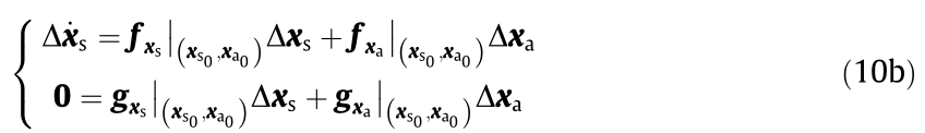
where and  respectively represent   and . Define , , , and . Thus, the system shown in Eq. (10b) can be expressed as follows:

When matrix is non-singular, can be eliminated; Eq. (10c) can then be simplified as follows:

Note 1: Based on Eq. (10d) and nonlinear system theory, we can have the following important concepts:

(1) For the system defined by Eq. (10), when matrix is non-singular, if and only if all eigenvalues of matrix  have negative real parts, the system is small-disturbance stable at  ; when matrix   is non-singular and the eigenvalues of   vary continuously with  , if any real eigenvalue of  is changed from negative to positive, the point  corresponding to = 0 is called a SNB of the system and, after this point, the system will lose stability in a monotonic mode when there are some small disturbances.

(2) If the real parts of a pair of conjugate eigenvalues  change from negative to positive, the point  corresponding to   is called a Hopf bifurcation (HB) of the system defined by Eq. (10) and, after this point, the system will lose stability in a continuous oscillation mode with increasing magnitude when there are some small disturbances.

(3) The matrix is not always non-singular, and may be singular in some cases. If is singular, it will be impossible to eliminate  from Eq. (10c); thus, it will be impossible to obtain Eq. (10d). In this case, the point that makes singular is called as singularity-induced bifurcation (SIB) of the system defined by Eq. (10). At this point, has a real eigenvalue μ , which changes its sign at the SIB. When μ crosses the zero point,  will have an eigenvalue k that changes its sign suddenly from infinity at one end to infinity at the other end (i.e., or 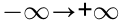 ). If matrix   has an eigenvalue that changes suddenly from , the system will lose stability in a monotonic mode when there are some small disturbances.

Hence, in the power injection space (i.e., parameter space) R²ⁿ , the SR to ensure the small-disturbance stability of the system defined by Eq. (10) is defined as follows:

The research on the boundary of Ω_SD (denoted by ) also involves the chaos phenomenon [19–22] in addition to the SNB, HB, and SIB. About the boundary of SDSR and chaos in power systems, Fact 4 was found.

Fact 4. Chaos occurs outside the bifurcation boundaries of the SDSR.

Remark: According to Ref. [21], the chaos phenomenon in power systems is formed by further development of singleperiod bifurcation, and is likely to be an intermediate stage of large-disturbance instability. Several ways of instability and collapse induced by chaos are shown in Fig. 6. If (based on Hypothesis 2) the boundary of the SDSR is the boundary that is first encountered during outward extension (i.e., the gradual increase of the system load) from the normal operation point in the power injection space, the chaos phenomenon will occur only outside the HB boundary of the SDSR in power systems (i.e., chaos will not occur in advance of HB). Since HB is not allowed in the secure and stable operation of power systems, there is no need for further research on chaos. Then, if non-periodic instability caused by SNB or SIB corresponds to the boundary that is first encountered during outward extension from the normal operation point in the power injection space, and if no single-period oscillation of HB occurs, no chaos will occur. Therefore, chaos does not need to be investigated too much in SDSR research, thus greatly reducing the search range of Ω_SD.

《Fig. 6》

Fig. 6. Several ways of instability and collapse induced by chaos. Q_1d: the reactive power load; K_A: proportion coefficient of the excitation system; T_A: time constant of the excitation system.

After excluding the consideration of chaos, it is also noted that the definition shown in Eq. (11) does not assume that is not singular, so the boundary of Ω_SD can be formulated as follows [23]:

where  is the closure of , and SIB only occurs under special load.

In addition to the abovementioned SNB points defined by the dynamic equations shown in Eq. (10), the SR boundary  consisting of SNBs also includes the singular point of the power flow Jacobian matrix. In practical engineering analysis, singular points are usually found using the continuous power flow (CPF) method with a single parameter variation, and are customarily called fold bifurcation points, while the corresponding boundary is called the boundary of power flow feasible region. The boundary of the SR to ensure static voltage stability (see Note 2) is of particular concern in power systems and it belongs to this kind of boundary. As mentioned earlier, the SR to ensure static voltage stability in the power injection space is abbreviated to SVSR and the SR to ensure static voltage stability in the corresponding cut-set power space is abbreviated to CVSR.

Note 2: In recent years, static voltage stability has been of great concern in power systems. There are two definitions of voltage stability. One definition is given by the Conseil International des Grands Réseaux Électriques (CIGRE) working group on voltage stability. This definition is based on the small-disturbance stability bifurcation theory, and thus belongs to the category of the abovementioned small-disturbance stability SR. The other definition, which is also commonly used, is given by the Institute of Electrical and Electronics Engineers (IEEE). Voltage stability is defined as the capability of a system to maintain its voltage. When the load admittance increases, the load power increases accordingly, and both the power and the voltage are controllable. As shown in Fig. 7 [7], for general ZIP static load models (where Z stands for constant impedance, I stands for constant current, and P stands for constant power), the SNB (i.e., singular point of the power flow equation’s Jacobian matrix) of the system is located at the lower half branch of the P–V curve. An increase in load admittance will lead to a decrease in load power in the lower half branch of the P–V curve. According to the IEEE’s definition of voltage stability, the lower half branch belongs to the unstable region. Therefore, only the upper half branch of the P–V curve is considered, and the nose tip of the P–V curve (i.e., fold bifurcation) is taken as the critical point of the static voltage stability. This nose tip is also the system SNB point obtained in the constant power load model. Therefore, only the constant power load model needs to be considered in the calculation of the static voltage stability SR.

《Fig. 7》

Fig. 7. Singular point on the P–V curve [7]. ① System P–V curve; ② characteristic curve of ZIP load model; ③ characteristic curve of constant power load model.

In regard to , the following two facts are found:

Fact 5. Not all SNB points are on the SDSR boundary .

Remark: Through bifurcation analysis and the two-step analysis method, the following conclusions are given in Ref. [24]:

(1) Considering the recoverable dynamic load while ignoring the dynamics of other components such as generators, the system voltage stability limit point obtained from small-disturbance analysis—that is, the SNB point—is the same as the fold bifurcation point obtained based on the CPF of the static constant power load model (the nose tip of the P–V curve). That is to say, the boundary of the power flow feasible region coincides with the SNB boundary of the SDSR. When the specific dynamic load and the dynamics of the generator and its regulating systems are considered, it is probable that the SNB point will occur in advance of fold bifurcation. In other words, the SNB points of DAEs might still exist in the power flow feasible region, i.e., the SR to ensure the existence of EPs.

(2) These SNB points will not necessarily cause voltage collapse in power systems. Not all SNB points are on the boundary of the SDSR. The nature of SNB points needs to be analyzed according to the specific conditions of the system. When induction motors (IMs) account for a large proportion of the load, it is essential to judge the nature of SNB points by means of a time-domain simulation when determining the boundaries of the SDSR.

Fact 6. The presence of IMs in the load might lead to no occurrence of HB in power systems before the increase of power injections causes voltage instability of the SNB type.

Remark: In theoretical research, HB generally occurs in advance of the SNB point. However, this type of voltage oscillation instability phenomenon is seldom discovered in the actual recording of voltage instability events. The voltage instability of actual power systems is often in a collapse mode with a monotonic voltage drop, which is closely related to SNB. In the opinion of some scholars, the occurrence of monotonic voltage collapse before reaching the HB of an unconstrained system might be caused by the operation limits in power systems. This is called limitinduced bifurcation (LIB); thus, no HB occurs on the SDSR boundary. However, in reality, many voltage instability events are not necessarily caused by the operation limits of the system. According to Ref. [24], the presence of IMs might lead to no occurrence of HB, and the voltage oscillation phenomenon resulting from HB before SNB-type voltage instability is caused by the increase of power injections. Therefore, when there is a high proportion of IM load in the system, SNB can be prioritized instead of HB.

Fig. 8 provides the voltage stability limit and the relationship between instability modes and the proportion of IMs in the load. On the one hand, the figure shows the particularity of the IM load model in voltage stability limit calculation, such that HB will not occur due to the increase in the proportion of IMs in the load. On the other hand, the figure indicates that there is a big difference between the result of CPF based on static models (fold bifurcation) and the more accurate result of small-disturbance voltage stability analysis based on dynamic models (SNB point) and the SNB points of the DAE system are still likely to exist in the power flow feasible region (i.e., the SR to ensure the existence of EPs).

《Fig. 8》

Fig. 8. (a) Voltage stability limit and (b) the relationship between instability modes and the proportion of IMs in the load.

《3.3. DSR (Ωd) to ensure transient stability》

3.3. DSR (Ω_d) to ensure transient stability

The DSR [7,13] of a power system in power injection space is defined as follows:

where F_d is a given fault; i_d and j_d are the pre-fault and post-fault network topology, respectively; represents the system state at the instant of fault clearing ; and represents the stable region encircled by EPs in the post-fault injection space. Both and are determined by . It should be noted that Ω_d determines a set of all points in the pre-fault power injection space that can ensure the transient stability of the power system.

In research on transient stability with direct methods, one injected power vector (an operation point) will correspond to a transient stability region [19,20]. Fig. 9 [18] shows the distinction and correlation between the DSR Ω_d and the transient stability region .

《Fig. 9》

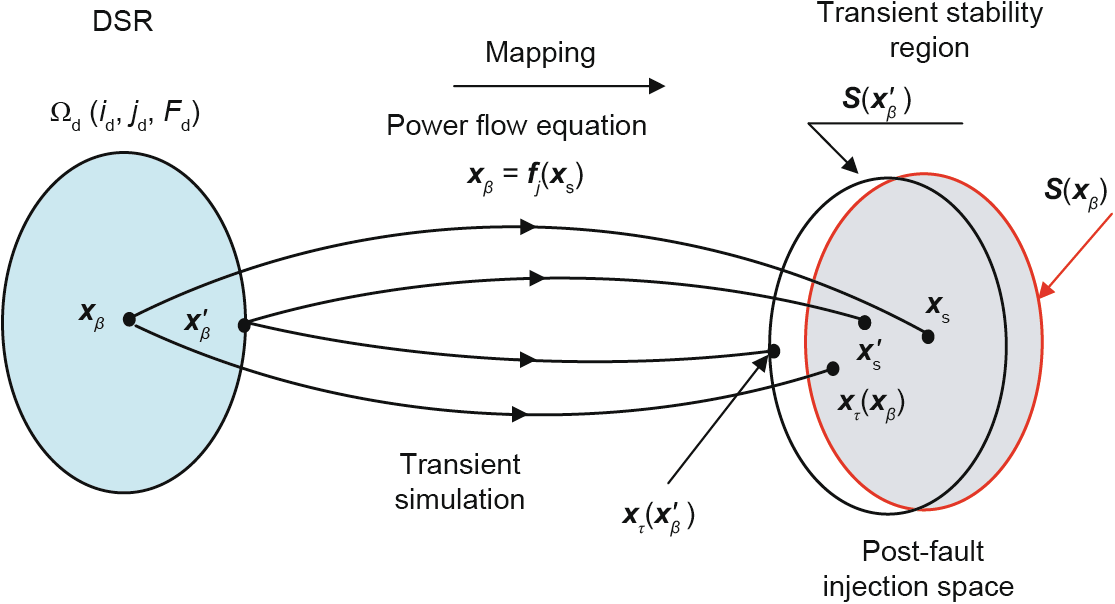
Fig. 9. Correlation between the DSR and the transient stability region [18].

After the fault is cleared, if in the group of generators with relative accelerations that are equal to zero in the generator rotor swing equations and phase angles that are greater than π/2, there are some generators with a relative speed of changes in the phase angles that is still greater than zero, such generators will be out of synchronization with the others, and the power system will not be able to recover to synchronous operation. In general, the set of generators with phase angles greater than π/2 is called an unstable generator group, while the set of other generators is called a non-unstable generator group. The different classifications of the unstable generator group and the non-unstable generator group are called different instability modes in this paper.

It is well-known that the transient power angle instability mode of a power system is closely related to the controlling unstable EP (CUEP). The post-fault trajectory of the system evolves along the unstable manifold of the CUEP. Considering that the power system’s loss of transient power angle stability is always accompanied by a sharp and excessive increase of the branch angle in certain or some critical cut-sets of the power system, it has been realized that the critical cut-set (see Note 3) in the power system is equivalent to the unstable EP (UEP) of the system, and the cut-set stability criterion has been put forward. To enable researchers to correctly apply the stability criterion related to the critical cut-set, the following fact has been proved theoretically in Ref. [25]:

Fact 7. If the CUEP of transient power angle stability is k-type, there will be k corresponding critical cut-sets in the network.

Note 3: If there is a cut-set in a network and the absolute values of all branch angles (radian) in this cut-set are greater than π/2, this cut-set is called a critical cut-set and the branches comprising it are called saturated branches. An individual critical cut-set divides the whole network into two connected sub-graphs, which correspond to two node groups, respectively. Of these groups, the one in which the voltage phase angle of the nodes is obviously larger is defined as a critical node group, and the other one is called a non-critical node group [25]. So, a critical node group contains— and only contains—generators in the unstable generator group.

Remarks: The correspondence is as follows:

(1) Most of the UEPs in a system are 1-type. If the CUEP of a system is a 1-type hyperbola (see Note 4), there must be a unique critical cut-set in the network that will separate the system into two parts: a critical node group and a non-critical node group, which correspond to the unstable generator group and the non-unstable generator group, respectively.

(2) If the CUEP in a system is an k-type hyperbola, there must be k critical cut-sets in the network corresponding to it. These critical cut-sets separate the system into k critical node groups (i.e., k unstable generator groups) and one non-critical node group (i.e., one non-unstable generator group). The CUEP corresponds to k instability modes.

Fig. 10 gives an example of the relationship between the transient instability mode and the critical cut-set in a system of four generators and 11 nodes. In the case of a fault on branch 6–9 (which refers to the branch between bus 6 and bus 9 in Fig. 10(a)), instability among three groups will occur in the system. The CUEP of this instability mode is 2-type and, in the corresponding system, there are two branches (i.e., branch 10–8 and branch 7–5) whose angle differences are sharply changed in separate direction to form two critical cut-sets.

《Fig. 10》

Fig. 10. Diagram of (a) a four-generator 11-node system and (b) the angle difference curve after a contingency.

Through Fact 7, the pure mathematical concept of the CUEP is linked with the physical properties of a network, thus providing useful information for the analysis of complex instability modes of power systems from the perspective of network topology. Based on this fact, the cut-set stability criterion can be easily extended to the multiple generator group instability. A modified cut-set stability criterion has been established to eliminate the conservatism of the original cut-set stability criterion [14].

Note 4: The basic types of EPs can be identified by the local linearized expression of the dynamic system near these points. That is, the stability type of an EP can be decided by the eigenvalues of its linearized dynamic matrix. If there is no eigenvalue whose real part is zero, the number of eigenvalues with positive real parts will be regarded as the exponent of this EP. If this exponent is equal to zero, this EP is stable in linear approximation and is generally referred to as a stable EP (SEP). If this exponent is equal to i , this EP is called an k-type UEP (UEP-k). In general, an EP can be called a hyperbolic equilibrium point only when all the eigenvalues of the local linearization of the dynamic system have no zero real parts [7].

4. Topological and geometric characteristics of SRs and methods to determine SR practical boundaries

As mentioned above, the most basic issues for power system security and stability identification include power flow stability, transient stability, static voltage stability, and low-frequency oscillation stability. Therefore, this section will introduce the topological and geometric characteristics of SRs and methods to determine their practical boundaries.

Based on Hypothesis 1 and Hypothesis 2, four important facts about the boundaries of the above SRs in real power systems have been found through a great deal of simulation research and theoretical analysis.

Fact 8. The SSSR, Ω_SS, which is defined in the power injection space and the decision space to ensure the power flow security of transmission and distribution networks, is the intersection of Ω_T (the thermal stability SR to ensure the thermal stability constraints (THSR)), Ω_V (the steady-state voltage SR to ensure the node voltage magnitude constraints), and the region constrained by the equipment capacity limits. For a given network topology and system component parameter i_s , the SSSR Ω_SS (i_s) is uniquely determined, connected, and void-free, and does not change with operation states. From an engineering perspective, both Ω_T and Ω_V can be described approximately by a hyper-polyhedron, and their boundaries can be described as pairs of HPs. The region between each pair of HPs respectively corresponds to the thermal stability SR of a given line or the steady-state voltage SR of a given node. Such an SSSR is called a practical SSSR (PSSR) in this paper.

Remarks:

(1) In 1989, the thermal stability SR was studied in active current injection spaces based on the decoupled power flow model [11], in which the affine relationships between node voltage angles and branch angles (i.e., the difference of voltage phase angles at both ends of the branch) are used, and the maximum allowable value of line angles is used to approximate the maximum line current magnitude. Meanwhile, all node voltage magnitudes of the system should be known in order to generate the mathematical expression of the SR. In the three-node system shown in Fig. 11(a) [11], node 0 is the reference node and its complex voltage is . With the given node voltage magnitudes V = (V₁, V₂) ^T , the angle differences between the two endpoint nodes (θ₁–θ₀, θ₂–θ₀, θ₁–θ₂) is proportional to the active power of lines 1–0, 2–0, and 1–2, respectively. On this basis, an affine transformation relation can be established between (h1, h2) and the node active current injections (which are proportional to the node active power injections). For the affine transformation shown in Fig. 11 [11], the preimage is the rectangle and the image becomes the parallelogram. Here, the image is the thermal stability SR in active current injection spaces, each pair of edges in the parallelogram corresponds to the thermal stability boundaries for the line currents in the forward and reverse directions, and the region between two parallel edges is the thermal stability SR for the line current.

《Fig. 11》

Fig. 11. Affine transformation diagram. (a) The three-node system; (b) the thermal stability SR in the voltage angle space; (c) the thermal stability SR in the active current injection space. TB: tree branch. The expressions and  are given in Ref. [11].

Then, the affine transformation shows the following characteristics [11]: ① The image and the preimage are in one-to-one correspondence, including the vertex, side, edge, and internal point; ② the images of parallel edges are still parallel edges; and ③ the images of parallel planes are still parallel planes. When the above conclusions are applied to a system with n₁ nodes (excluding the reference node), if the node voltages in the decoupled power flow model Eq. (2a) are specified, it can be seen that the thermal stability SR of power systems can be approximately expressed as the convex hyper-polyhedron enclosed by n_b parallel HPs in n₁- dimensional Euclidean space, each pair of HPs corresponds to the thermal stability boundaries for a line current in the forward and reverse flow directions, and the region between two HPs is the thermal stability SR of the line current. These features make the form of the SSSR boundaries concise. Even when studying the SR based on the AC power flow, these features are beneficial for understanding the entire SR. In addition, based on the ideology of affine transformation, Ref. [12] has studied the steady-state voltage SR in reactive current injection spaces.

However, because the above method simplifies the power flow model and line current constraints, and does not consider the relationship between the active and reactive line currents, there is an obvious error between the generated HP boundary and the real SR boundary.

For convenience in the description, the AC power flow equation Eq. (2d) is rewritten as in the following. Obviously, is continuous nonlinear mapping, and the preimage (i.e., the definition space of  is a hypercube defined by Eqs. (7a)–(7c). Under this mapping, ① the image of the vertex of the hypercube is a vertex; ② the image of the edge (straight line) of the hypercube is an edge, but not a straight line; ③ the image of the boundary of the hypercube is a continuous (smooth) curved surface, but not a HP; and ④ the images of the hypercube that is internally free of void are still free of void. Therefore, it can be concluded that, strictly speaking, the SSSR defined by the AC power flow equations is a polyhedron enclosed by several smooth hypersurfaces and is internally free of void.

(2) Ref. [26] examines the calculation method for the thermal stability SR in decision spaces. Based on the AC power flow model and the sensitivity method, the proposed method successively generates the mathematical expression of the corresponding thermal stability SR boundaries for each line . The boundaries are pairs of HPs, and each HP corresponds to the critical current limit in one direction. The method to determine HPs is also provided in Ref. [26]. This method involves searching for a reference critical point on the boundary, which is the first encountered point on the SR boundary when continuously extending outwards from the initial normal operation point . It can be seen that this method satisfies Hypothesis 2. Then, the thermal stability SR of the entire power system is the intersection of the thermal stability SR of all lines:

It should be noted that the HPs in pairs are no longer strict parallel planes, as described in the affine transformation in Remark (1).

Ω_T in Eq. (14) is a hyper-polyhedron surrounded by n_b pairs of HPs in a 2n-dimensional decision space, and has a very complex shape. However, because the number of overload lines (which belong to a set ) in the real power grid is limited within a certain period, and the overload current direction can be known, we can only focus on the corresponding thermal stability SR in some given current directions.

The method described in Ref. [26] can also apply to fast calculation of the steady-state voltage SR Ω_V, which ensures the node voltage constraint in decision spaces. The steady-state voltage SR of the entire power system Ω_V is the intersection of all nodes 

Each  has a pair of HP boundaries that correspond to the upper and lower limits of the voltage at node i , respectively. Therefore, Ω_V is the hyper-polyhedron surrounded by 2(n – n_g) HPs in 2n-dimensional decision spaces. The method to determine the HPs of boundaries is given in Ref. [7].

Thus, the SSSR of the entire power system can be obtained by the intersection of the thermal stability SR of all lines Ω_T and the steady-state voltage SR of all nodes Ω_V:

Eq. (16) is expressed as many simultaneous linear inequalities, and can be easily dealt with by computers.

(3) The above references mainly focus on the SSSR of transmission networks Ω_SS. For a distribution network, since it uses the same power flow model as that of transmission networks, they likely have the same abovementioned characteristics. Indeed, in Refs. [27,28], it is demonstrated that Eqs. (14)–(16) can also be used to define the steady-state voltage SR and the thermal stability SR in power injection spaces of the distribution network, and that a pair of HPs can also be used to describe the corresponding SR boundaries (such kind of characteristics are consistent with the transmission network). The difference is that Refs. [27,28] propose simple generation methods for the SSSR based only on the radial topology of distribution networks, and HP coefficients can be directly generated by using the network topology and line impedances. The simulations show that the proposed methods are fast enough to meet the needs of a distribution network with frequent changing topologies. By combining these generation methods of SRs in distribution networks with the abovementioned generation method of SRs in transmission networks, coordinated optimization of transmission and distribution networks can be executed effectively. Considering that the loads, distributed generations, and energy storages can be expressed as power injections, this research can be used in the monitoring, optimization, and security assessment of smart grids. (Specific application examples are given in Section 5.) Ref. [29] examines the thermal SR of distribution systems. Under the assumption that the node voltages are specified, SRs are used to describe the relationship of the power flows in radiant distribution networks and are applied to evaluate the distribution network security.

(4) Because the Ω_SS(i ) defined in this paper satisfies Hypothesis 1 and Hypothesis 2, the boundary of Ω_SS(i_s) is uniquely determined and connected for a given network topology and given system component parameters in the space defined by . Furthermore, Ω_SS(i_s) is internally void free due to the continuity of the region restrained by Eqs. (7a)–(7c) and the power flow mapping .

(5) Each HP of the SSSR in the form of a hyper-polyhedron can be described by the following equation:

where and are constant coefficients, and m_s is the total number of SR boundary surfaces. Because the SSSR is connected and uniquely determined for a given network topology and given system component parameters, and is irrelevant with the system operation states, all HP coefficients can be calculated offline and stored for online security monitoring, assessment, and optimization.

Fact 9. For a given network topology, system component parameters, pre-fault graph i_d, post-fault graph j_d, and fault F_d, the DSR Ω_d(i_d, j_d, F_d) defined in power injection spaces is uniquely determined and connected, and does not change with the operation states. Also, it is internally void free, and its boundaries Ω_d(i_d, j_d, F_d) may consist of a finite number of smooth subsurfaces, each of which corresponds to a specific instability mode. Each sub-surface can be approximately described by an HP within the scope of practical engineering. The DSR described in such way is called the practical DSR (PDSR) in this paper.

Fig. 12 shows the diagram of the New England 10-machine 39- node system and the cross-sections of its PDSR in three 2D spaces. The PDSR corresponds to the three-phase grounding short-circuit fault on bus 26 of lines 26–29. The duration of the fault is = 0.1 s, and the fault is cleared by disconnecting lines 26–29.

《Fig. 12》

Fig. 12. The diagram of the New England 10-machine 39-node system and the cross-sections of its PDSR in three 2D spaces. (a) The diagram of the New England 10-machine 39-node system; (b) PDSR in the active power injection space of G8 and G9; (c) PDSR in the active power injection space of G9 and L29; (d) PDSR in the active power injection space of G8 and L28. The line from M to N is the transversal of the critical HP of the PDSR in the 2D space. The active power limits of generators are shown as dotted-lines.

Remark:

(1) In 1990, by fitting a large number of transient stability critical points obtained by simulation, the authors of Ref. [13] first discovered that the PDSR boundary in the power injection space of the pre-fault system, which is shown in Eq. (8e), can be approximately described by a critical HP around the “basic operation point” in the scope of practical engineering application. The critical HP can be expressed as follows:

where is the constant coefficient of the HP expression and (P₁, ... ,P_n) is the critical active power vector in the power injection space of the pre-fault system, which ensures the transient power angle stability. Customarily, if < 1,  the system is considered o be transient stable, while  > 1 means that the system is transient unstable.

The absolute value of the HP coefficient represents the influence of the corresponding node power injection on the system stability. The positive or negative value of the HP coefficient represents the influence trend of the corresponding node power injection on the system stability; that is, an increase of the node power injection with a positive coefficient will deteriorate the system stability, while an increase of the node power injection with a negative coefficient will improve the system stability.

The discovery of these characteristics is of great significance because the linear combination constraint in the power injection space, which is shown in Eq. (18), is of great advantage in mathematical processing for power system assessment, operation, and control.

In Ref. [13], the potential energy boundary surface (PEBS) method [7] is used to find the critical injection vector, and then the HP coefficient in Eq. (18) is determined by the leastsquares fitting method. Ref. [13] recommends the use of the quasi-orthogonal method to select possible searching directions in order to achieve uniform distribution of critical points, which can reduce the number of required critical points and ensure accuracy.

(2) In Ref. [30], the 984-node system of the Central China Power Grid is used to validate the proposed method, considering the dualaxis reaction of the generators, the excitation system and the speed governing system, features of the IMs, and the static var compensator (SVC). Using transient stability simulation tools, a great number of critical points on the DSR boundaries are searched through numerical simulations. The authors further prove that the DSR boundary for transient power angle stability can be approximately described by an HP via least-squares fitting. Each critical point is the SR boundary point that is first encountered by continuous outward expansion from the initial normal operation point along different ray directions in the active power injection space, as shown in Eq. (8e).

(3) The least-squares fitting method requires approximately 2n suitably distributed critical points. It can only be calculated offline and then used online due to the great amount of calculation required, although highly accurate SR boundary coefficients can be obtained. To solve this problem, the analytical expressions of the HPs of the PDSR boundary are derived in Refs. [31,32] based on the structure-preserving model of a power system, as well as the sensitivity of the initial operation state, the operation state at fault-clearing time, and the energy function to the node power injections. Based on the fact that the Gramian matrix of the power system dynamic model at the short-circuit fault-clearing time remains almost unchanged compared with the Gramian matrix of the power system dynamic model near the initial operation point, Ref. [33] proposes a method, that combines coherency identification based on k-medoids method with the initial acceleration, to rapidly identify the transient instability mode (and thus to identify the critical cut-set) near the initial operation point.

(4) In order to provide a theoretical basis for the application of the DSR, Ref. [34] has proved the following characteristics of the DSR based on the differential topology theory for the structurepreserving model of power system transient stability analysis [20] of a power system: ① The DSR determined by the CUEP method is internally void free, that is, showing density; ② (i_d, j_d, F_d), the boundary of the DSR, will not knot—that is, it is not torsional or expansive—and the local surface corresponding to the same instability mode k_d is continuous; and ③ the boundary of the DSR is compact—that is, it can be expressed by the union set of a finite number of sub-surfaces, and each critical sub-surface corresponds to a different instability mode.

(5) According to Fact 7, when the CUEP of the system is an i-type hyperbola, there must be i critical cut-sets in the corresponding network, that is, there must be i instability modes in the system corresponding to the CUEP. Therefore, the corresponding (i_d, j_d, F_d) must have i sub-surfaces, each of which corresponds to an instability mode.

(6) Furthermore, the cut-set power space can be used to simplify the description of the DSR. However, the SR in the cut-set power space is not unique, as it is not defined in the -defined space (see Fact 2). As indicated by studies on the DSR in a cut-set power space (CDSR) in Refs. [35,36], for a given network topology and given system component parameters, the total transfer capacity (TTC) in the critical cut-set of the system is relevant to the operation states (power injection vector), that is, the CDSR is not uniquely determined. For this reason, it is necessary to seek the maximum value of the TTC, by which the HP of the PDSR in the power injection space can greatly reduce the computational burden. However, the boundary of the CDSR may vary in a small range and can be used approximately in a few practical scenarios.

(7) A large number of simulation studies in Ref. [37] show that, for a large number of different (i_d, j_d, F_d), all (i_d, j_d, F_d) can be approximately expressed by the following HP in a complex power injection space defined by Eq. (8c) [7]:

If the changes in both the node active power injections and the node reactive power injections are considered, especially when involving the transient voltage stability, Eq. (19) will have a better accuracy. According to Ref. [37], the boundary of the PDSR in the pre-fault power injection space has the approximate translation property in the case of a change in the proportion of the IMs in the load. Therefore, the interpolation method can be used to determine the DSR boundary under different proportions of IMs in the load.

For the load that consists of both constant impedance loads and IMs, transient stability simulations show that the critical faultclearing time of the transient stability is closely relevant to the proportion of motors in the load, and the increase of the proportion of motors in the load will result in the decline of the critical faultclearing time. In addition, the system transient instability mode mainly manifests as transient voltage instability when the proportion of motors is high and as transient power angle instability when the proportion is low, as shown in Fig. 13.

《Fig. 13》

Fig. 13. Relationship between the transient instability mode and the proportion of IMs in the load.

(8) Ref. [38] shows that, for an alternation current (AC)–DC hybrid transmission system, the critical HP description of the PDSR in the decision space still has good accuracy. The boundary equation of the PDSR corresponding to a certain instability mode can be expressed as follows:

where G and L are the set of generator nodes (except equilibrium nodes) and the set of load nodes, respectively; V_i is the voltage of generator node i ; and  and μ are the critical HP coefficients of the PDSR. , where sb and rb are the number of AC nodes at the sending end and the receiving end of the DC line, respectively. Therefore, the DC power P_d can be regarded as an active power variable of the critical HP equation. Under the same failure mode, instability mode, and DC control mode, all the critical HPs corresponding to different DC power have approximate parallelism, and the spatial geometric distance between them is approximately proportional to the change in DC power.

(9) Ref. [39] examines the DSR of a power system with doublyfeed induction generators (DFIGs). The accuracy of its boundary is verified through time-domain simulation. The DSR of a power system with photovoltaic (PV) generation is calculated in Ref. [40]. According to Refs. [39,40] and within the engineering perspective, the boundaries of the PDSR in the power injection space can still be approximately described by HPs for a power system with DFIG or PV generation. Ref. [39] also analyzes the influence of the integration of DFIGs on the DSR, and finds that the integration of DFIGs would cause external expansion of the DSR in a power system.

Fact 10. For a given network topology and given system component parameters, the SVSR in the power injection space corresponding to fold bifurcation is uniquely determined, connected, internally void free, and does not change with the operation states. Furthermore, its boundaries are smooth. When the load node power injections are specified, the boundary of the SVSR in the generation power injection space can be approximately expressed by an HP in the practical engineering range. When there is only one critical cut-set in the system, CVSR can be approximately described by an HP within the practical engineering range (as shown in Fig. 14). When several critical cut-sets should be considered in the system, the boundary of the CVSR corresponding to each critical cut-set can be approximately described by an HP within the practical engineering range. In addition, the union set of the boundaries of the CVSR of all cut-sets is the boundary of the CVSR under a given network topology and given system component parameters.

《Fig. 14》

Fig. 14. Local diagram of a real power system and boundary of the CVSR on critical cut-set marked by dotted lines. (a) The diagram of a real power grid; (b) the boundary of CVSR in a 3D power injection space.

Remarks:

(1) In Ref. [41], since the voltage stability problem has strong local characteristics, the voltage stability boundary can be approximately described by the injected power of the nodes with weak voltage stability in the system. Its relatively complex boundaries can be visualized by an artificial neural network. In Ref. [42], a quadratic polynomial is used as an approximate analytical expression for the large-scale boundaries of the SVSR in active and reactive power injection spaces. Meanwhile, in order to reduce the dimension of the power injection space, the key nodes of the system are selected by using modal analysis. A large number of simulation results show that this method has satisfactory engineering accuracy. In Ref. [43], an approximate analytical expression of the SVSR boundary is constructed by the eigenvalue sensitivity and eigenvector sensitivity of Jacobian matrix. Although the precision of this method is higher than that of the HP-based linear approximate expressions, it is far less convenient than the HP method when applied in optimization and risk analysis.

(2) Ref. [44] is based on the power flow feasible solution region. It takes whether the power flow equation has a solution or not as the decisive factor of the SSSR by using a new “hybrid method” for feasible region boundary computation, proposed by the authors in Ref. [45]. With a prediction–correction ideology and optimization technique, this hybrid method takes into account the limit of the system equipment while tracking the boundary of the power flow feasible region composed of singular points of the Jacobian matrix of the power flow equation (fold bifurcation) and LIB. In Ref. [44], the power injection space is divided into the load injection space and the power generation injection space. By fitting a large number of critical points obtained by static voltage stability simulations, it can be found that the boundaries of the power flow feasible region in the above two sub-spaces have distinct geometric characteristics. In the power generation injection space with a specified direction of load growth, a part or the majority of the boundary of the power flow feasible region can be well approximated by an HP in the practical operation range, as shown in Fig. 15 [24]. Another new algorithm is put forward in Ref. [44] to track the farthest (L1 norm) boundary point of the power flow feasible region in the high-dimensional power generation injection space, which avoids the frequent start of CPF calculation. The multi-solution of the results is also used to further verify that the boundary of the power flow feasible region can be approximated by an HP.

《Fig. 15》

Fig. 15. View of 2D transects (see Note 5) of the power flow feasible region of IEEE 118-bus system in a power generation injection space [24].

Note 5: Because the vector of power generation has a very high dimension, an SR as whole is difficult to visually represent. Therefore, the above figures show only the transects of the SR of concern in a 2D power generation space. All transects are obtained by supposing that the variables other than the given coordinate variables remain unchanged. If the edge lines of the transects all appear as straight lines in a large range of actual engineering concerns, then it can be inferred that, in a high-dimensional space, the boundary surface of SRs can be approximated by an HP in a large range of engineering concerns.

(3) Ref. [46] provides a local visualization method for the steady-state voltage stability region in the cut-set power space based on the ideology of the power flow feasible region. Refs. [47,48] clearly propose that the practical boundary of the CVSR can be approximately described by Eq. (21) with an HP expression:

where C indicates the critical cut-set, P_L,i is the active power flow of line i in the critical cut-set, and Q_L,i is the reactive power flow at the sending end of line i in the critical cut-set. Conventionally, if  < 1, the system is considered to satisfy the steady-state voltage stability constraint, while if  > 1, the system is considered to be steady-state voltage unstable, as shown in Fig. 14.

In Fig. 16, a method to quickly determine the HP of the CVSR boundary is presented. First, the CPF is used to find a SNB point of the system. Then, the tangent plane of the SVSR boundary at the SNB is represented by the eigenvector at the critical point. Finally, the critical boundary of the CVSR with an HP expression is obtained by the transformation from the power injection space to the cut-set power space.

《Fig. 16》

Fig. 16. A method to determine the HP of the CVSR boundary. Pg: a critical point on the boundary of the SVSR.

(4) When there is a large error, some power injections of nodes with weak voltage stability at the receiving end of the system can be used as additional variables of Eq. (21) to improve the fitting accuracy.

(5) Considering that the number of lines in the critical cut-set is very limited, the HP coefficients and can be obtained by the least-squares fitting method after finding about 4n_c (where n_c is the total number of lines in the critical cut-sets) appropriately distributed critical points through simulation. Based on this method, a software to determine the CVSR has been developed and the results show that the software can meet real-time online needs in practice [48].

(6) In some systems or cases, the weak nodes of the system may be distributed in different areas, which requires multiple critical cut-sets [46]. Therefore, all the operation points that ensure static voltage stability are in the region defined below:

where are the msv critical cut-sets that need to be considered, and m_sv is generally a small integer.

(7) The statistical analysis in Refs. [48,49] shows that, under the actual possible load growth mode, the weak node sets in the system are concentrated in several areas and most of them are distributed at the terminals of long transmission lines without reactive power support. The graph model corresponding to the grid structure can be established according to the connection relationship and the degree of closeness between nodes. The spectral clustering algorithm can be used to determine the voltage stability area (the node set with weak voltage stability in the power system) and the critical cut-set (the potential critical cut-set) of the power system.

(8) Static voltage instability is based on the absence of power flow solutions, and the SR defined in this paper complies with Hypothesis 2; that is, the SVSR boundary is the first static voltage instability boundary encountered by continuous outward extension from the initial operation point. Then, along with the continuity of power flow functions , it can be concluded that the SVSR is uniquely determined, connected, and internally void free. Its surfaces are smooth in -defined space. The mapping of this region to the low-dimensional cut-set power space, that is, the CVSR, can retain these properties. Therefore, the CVSR in Fact 10 is also internally void free.

Fact 11. For a given network topology and given system component parameters, the SDSR, Ω_SD in the power injection space is bounded by SNB boundary ((SNB)) and/or HB boundary ((H)). It is uniquely determined, connected, and internally void free, and does not change with operation states. , the boundary of Ω_SD, is composed of several smooth surfaces, and the sudden change occurs at the junction between (SNB) and (H), or on (H) when its dominant oscillation mode changes. Each smooth surface can be approximated by an HP in a large range (as shown in Fig. 17 [50]), which can meet the practical engineering requirements. In this paper, the SR described in such a way is called a practical SR to ensure small-disturbance stability (PSDSR).

《Fig. 17》

Fig. 17. Piecewise fitting under multiple dominant modes (New England 10- machine 39-node system) [50].

Remarks:

(1) In the investigation of small-disturbance stability [21], the detailed evolution process from HB to chaos is demonstrated by an illustrative power system, and the law of increasing energy is revealed. It is also found that the boundary of the SDSR relevant to oscillatory instability can be described by the HB boundary (H), and that there is no need to account for more complex chaos.

(2) Ref. [50] shows that (H) in the active power injection space is composed of several smooth curved surfaces, each of which can be approximately described by Eq. (23), where the reactive power is assumed to be locally balanced:

where P_i is the injected active power at node i , is the HP coefficient of node i , and n is the total number of other nodes in the network without the reference node.

(3) (H) may be composed of one or several smooth surfaces, and the reason why the sudden change occurs at the junction among surfaces is that those surfaces have different dominant oscillation modes. Based on the above knowledge, Ref. [50] applies the following piecewise fitting strategy to obtain the approximate HP for (H). Eigenvalue analysis is first conducted for each critical point to determine its dominant oscillation mode. Then all the critical points are divided according to their dominant oscillation modes, and those with the same dominant mode are clustered into the same set. The critical points in each set can be fitted by an HP, and the union set of the fitting boundaries corresponding to all dominant oscillation modes constitutes (H) in the power injection space (as shown in Fig. 17 [50]).

(4) The influence of DFIGs on power system electromechanical oscillation is examined in Ref. [51], and it is found that the SDSR boundary of a power system with DFIGs is composed of several smooth surfaces, including (SNB) and (H) under different dominant oscillation modes. Fig. 18 [51] shows the 2D crosssection of a SDSR boundary in the active power injection space of two generators. When the active power output constraints are not considered, the boundary is composed of several smooth curves. Boundaries 1 and 3 correspond to HB, and boundary 2 corresponds to SNB. There are sudden changes at the junction between boundaries 1 and 2 and at the junction between boundaries 2 and 3. When the active power limits (shown as the rectangle in Fig. 18 [51]) of the generators are considered, the actual SDSR of concern is the shaded area. The appearance of SNB on boundary 2 is due to the fact that the excitation system of generator G4 reaches its limit, which is the LIB problem in Fact 5. Therefore, it is necessary to determine the boundary of an SDSR through time-domain simulation, as is described in Fact 10.

《Fig. 18》

Fig. 18. 2D section of an SDSR boundary [51].

(5) The uniqueness, connectivity, and the void-free characteristics of SDSRs can be proved in a similar way to those of Remark (8) in Fact 9, which will not be repeated here.

《5. Methodology of SR with its boundaries expressed by HPs for power system analysis》

5. Methodology of SR with its boundaries expressed by HPs for power system analysis

《5.1. Application of SR methodology in power system optimization》

5.1. Application of SR methodology in power system optimization

The power system optimization problem with security and stability constraints can be described by the following general model. Let be the optimization variable vector, which usually refers to the active/reactive output of generators or the active/reactive power of loads. is the optimization objective. Securityconstrained optimization problems of power systems can be described by the following general model, as Eqs. (25)–(30) show. The model will change with the specific scenarios of applications. For example, in security-constrained optimal power flow, the objective function usually considers the minimum power generation cost or loss, while in the security-constrained optimal control of power systems, the objective function usually considers the minimum control costs, such as the load shedding cost and so forth. is the equality constraint function, which mainly includes the power flow equations.  is the inequality constraint function, including the generator output limit, the node load constraint, and so forth. Eqs. (27), (28), (29), and (30) represent the node voltage constraint, power flow security constraint, small-disturbance stability constraint, and transient stability constraint, respectively.

V_i represents the voltage magnitude of node i ; I_i represents the current of branch i ; represents the ith eigenvalue of the system operation state; CTS represents the set of contingencies for the transient stability test; represents the difference of power angle between generator i and generator j at t in case of contingency k ; and represents the maximum allowable power angle difference between the generators.

The decision variable is usually the active/reactive output of the generators, that is, and . As shown in Eqs. (27)–(30), the inequality constraints also involve other variables, that is, which are not included in the objective function. In particular, V_i  and I_i are coupled to P_G and Q_G in the objective function via power flow equations, while and   are coupled to P_G and Q_G via power flow equations and differential equations. It is necessary to repeatedly solve power flow equations to verify whether the constraints shown in Eqs. (27) and (28) follow, repeatedly calculate eigenvalues of the system at the point corresponding to the power flow solution to verify whether the constraints shown in Eq. (29) follow, repeatedly solve a set of large-scale DAE (in a real power system, the dimension of the DAE may be several thousands and even tens of thousands), and simulate dynamic trajectories of the system during the optimization process to verify whether the constraints shown in Eq. (30) follow, which undoubtedly require an enormous calculation burden. As a result, the consideration of complicated security constraints such as transient stability constraint in the optimal power flow is always a difficult problem.

Based on SR methodology, those security constraints may be formulated as follows:

where  ≤ Const_j , , and  Const_r represent the constraints of the jth boundary of Ω_SS Ω_SV , the kth boundary of Ω_SD , and the rth boundary of Ω_d , respectively; and m_ss ,m_sd , and m_d represent the numbers of  and ,  respectively. The problem can be solved with quadratic programming (QP), which can save a considerable amount of calculation.

In particular, Eq. (31) can be further replaced by the following equations, when the SR boundaries are approximated by HPs:

In this equation,  are constant coefficients. The injected powers  of the load nodes are specified, while the  corresponding to each point  on the boundary is determined by the power flow equation. In this case, iterative calculations related to power flow may be needed. However, considering the low dimension of , the iterative calculation is much less.

Therefore, based on the fact that the boundaries of SRs in the power injection space can be approximated by HPs, system security constraints such as the power flow constraint, smalldisturbance stability constraint, and transient stability constraint can be formulated as explicit linear inequality functions of decision variables (i.e., node power injection), so that it will be extremely convenient to take into account various types of security constraints in power system optimization, and the calculation efficiency will be significantly improved.

Up to now, SR methodology has been widely applied to various power system optimization problems. For example, an optimization model of power system security cost in the electricity market is proposed in Ref. [52]. The transient stability constraint, fault probability, and system instability loss are considered by means of PDSR, through which optimal preventive control can significantly improve the economic efficiency of the power system. Ref. [53] reports on experiential laws about the parallelism and superposition of the critical surface of the extended PDSR. Based on this, it provides an optimal transient stability-constrained emergencycontrol method, and quantifies the control measures as cost indicators, which solves the problem of the difficulty quantifying the effectiveness of emergency-control measures. In Ref. [54], optimal active and reactive coordination of a power transmission system is realized considering security constraints based on SRs. By means of the SSSR, SVSR, and DSR, the power flow constraint, static voltage stability constraint, and transient stability constraint are considered comprehensively. Through the affine relationship between the active power and the branch angle of the power system and the affine relationship between the reactive power and the node voltage magnitude, an algorithm for solving the optimal power flow through QP is established, which significantly improves the calculation efficiency. In Ref. [55], the power flow constraint, steady-state voltage stability constraint, and transient stability constraint are, for the first time, simultaneously taken into account in the day-ahead dispatching of power systems, providing an important approach to solve the contradiction between security and economy in power system operation. In Ref. [56], models for the pricing of active and reactive power as well as corresponding solution algorithms are proposed, which systematically consider many complicated constraints, including quantification of transient stability in node pricing for the first time. In the proposed model, the static voltage stability constraint and the transient stability constraint are considered through the CVSR and PDSR, respectively, and a decoupled optimization and iteration method for active power production cost and reactive power production cost is suggested. Based on the marginal cost theory and Karush–Kuhn–Tucker (KKT) optimality condition, active power and reactive power are priced, respectively, and the component prices related to various security constraints are derived. In the proposed method, not only is it convenient to consider the contingency set, but this is also done with more concise expressions and clear physical meaning. In Ref. [57], SR methodology is adopted to establish static security and dynamic security value-based power system extension planning. In Refs. [27,28], the SR ideology is introduced into the reactive optimization of a power distribution network for the first time, providing a critical decision-making tool for the reactive voltage control of a smart power distribution network. An example of SR application with HP boundaries in the coordinated optimal power flow of a power system is provided here, as follows.

Example: SR application with HP boundaries in the coordinated optimal power flow of a power system with a given topology.

With increasing penetration of intermittent, fluctuating, and uncertain renewable distributed energy in smart distribution grids, transmission and distribution grids can affect the tie-line power by changing their own operation states. This means that it is necessary to consider the impact of tie-line power changes on each other’s operation state in both the transmission grid and the distribution grid. Hence, it is necessary to comprehensively consider the power generation resources in the entire grid for coordinated optimal power flow.

Nowadays, the methods for solving this coordinated problem can be mainly divided into two types. One type is the centralized optimization method [58]. Although this method can yield optimization results, it is necessary to collect and process the entire grid data during the application, and the difficulty of data maintenance and computation burden are very large. The other type is the distributed optimization method, which decomposes the coordinated optimal power flow problem of the entire transmission and distribution grids into several sub-problems for optimization. The solution speed of the latter method is faster than that of the centralized method [59]. However, the constraints in each subproblem include capacity constraint inequalities for devices, node voltage constraint inequalities, line current constraint inequalities, and AC power flow equations (similar to Eqs. (25)–(28)), and the decision variables in the objective function are power generation injections, which are nonlinearly related to node voltages and line currents based on power flow equations; thus, the determination process for each sub-problem and for the KKT conditions is still complicated.

In order to solve the problems in the existing methods, Ref. [60] applied the SSSR with HP boundaries to the optimal power flow problem of the entire transmission and distribution grids for the first time, and established a coordinated optimization method for the transmission and distribution grids. The characteristics of this method are as follows:

(1) The approximate HP expressions for the SSSR boundaries are generated based on the respective topological structure and boundary information of the transmission grid and the distribution grids in their power supply area. Considering that the SSSR is uniquely determined by the given grid topology and is irrelevant to operation states, for a transmission grid whose topology is relatively stable, the HP expression coefficients can be calculated offline and recalled online. For a radial distribution network, the HP expression coefficients can be generated online, which requires a small computation burden and can be fully adapted to the requirements of frequent changes in topology.

(2) In order to minimize the overall power supply cost of the transmission and distribution grids, SSSRs in the transmission and distribution grids are applied to describe the steady-state security constraints (as shown in Eq. (32)), and to establish the distributed optimization model for coordinated optimal power flow in the transmission and distribution grids; the boundary variables are shown in Fig. 19. During the execution of the proposed method, the transmission grid and distribution grids can complete the optimization only according to the boundary node voltage, the tieline power and the clearing prices (determined by KKT conditions) exchanged between the grids. Since the constraints become linear combination inequalities of decision variables, and the objective function is consistent with the variables in the constraints, the optimization process of each transmission grid and distribution grid and the determination of the KKT conditions become extremely simple.

《Fig. 19》

Fig. 19. Equivalent model of transmission and distribution grids. (a) Equivalent model of the entire grid; (b) equivalent model of transmission and distribution grids; (c) equivalent model of distribution grid k .

In order to verify the effectiveness of the proposed method, Ref. [60] first compares the proposed method with the centralized optimization method [58]. In the optimization process, the centralized method establishes a nonlinear optimization model based on an AC power flow model. The overall supply cost/calculation time obtained by the two methods is shown in Table 1. The optimization results obtained by the two methods are basically the same, but there are great differences in the calculation time.

《Table 1》

Table 1 Comparison of daily overall supply cost and calculation time (see Note 6).

Note 6:

(1) In order to briefly show the advantages of the practical SR boundary with HP expression in power system optimization, only the SSSR is considered in this example. If other security constraints are taken into account, the advantages of the SR methodology will be even more prominent.

(2) Case 1 is a modified IEEE 24-bus grid with nine distribution grids. Case 2 is a modified IEEE 118 with 20 distribution grids. Case 3 is a modified IEEE 300 with 40 distribution grids.

(3) Since the SSSR boundaries of the transmission grid are uniquely determined by the grid topology, they are independent of operation states, and the topology does not change frequently. Therefore, the coefficients of the SSSR boundaries can be calculated offline, stored in the database, and recalled according to the topology when used online. However, the coefficients of the SSSR in distribution grids need to be calculated in real time. Therefore, for the statistics of optimization time burden, the generation time of the SSSR in the distribution grid is included, and the generation time of the SSSR in the transmission grid is not.

The proposed method is then compared with the alternating direction method of multipliers method (ADMMM) [61] and the optimality condition decomposition (OCD) method [62], which are commonly used. The average optimization time consumed by the three methods in each iteration is shown in Table 2. It can be seen that since the proposed method is based on the SR method to establish the optimization models in the transmission and distribution grids, the variables in the objective function and the constraints are identical, and the constraints are linear combination inequalities of node power injections, so that the optimization speed of each sub-problem is fast.

《Table 2》

Table 2 Comparison of average optimization time in each iteration.

Furthermore, the average number of iterations required to complete a coordinated optimal power flow by the three methods is shown in Table 3. Since the Lagrangian multiplier corresponding to each constraint is needed in the process of determining the KKT condition, and considering that the constraints used in the optimization model of the ADMMM method and the OCD method are nonlinear and the constraints (i.e., the boundary HPs of SSSR) used in the proposed method are linear, the number of iterations varies greatly.

《Table 3》

Table 3 Average iteration times to complete a coordinated optimal power flow.

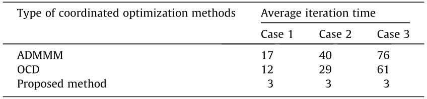
In summary, the total time required to complete the coordinated optimization of the entire transmission and distribution grid is mainly determined by the average optimization time consumed by each iteration of the transmission grid multiplied by the average iteration times to complete a coordinated optimal power flow. The proposed method has obvious advantages in both of the above factors, so that the average total time burden for coordinated optimization can be decreased by several orders of magnitude (as shown in Table 4).

《Table 4》

Table 4 Average total time for coordinated optimization. 

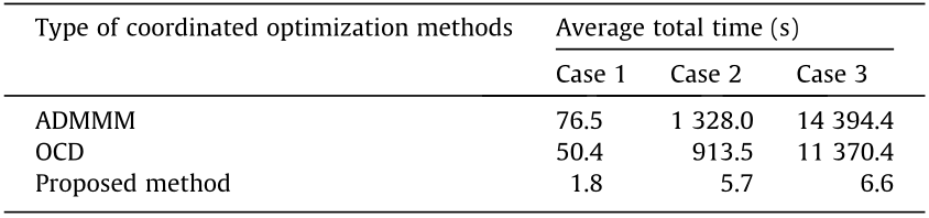
This example shows that the SR application with HP boundaries presented in this paper can successfully solve the problem of the security and stability constraints being difficult to deal with in a large class of power system optimization problems.

It should be noted that the average time consumed by the proposed method to generate the SSSR in the transmission grid is 1.67, 6.3, and 45.1 s for Cases 1, 2, and 3, respectively, showing that even if the average time for generating the SSSR of the transmission grid is included in the optimization time statistics, the superiority will not be affected when compared with the existing methods.

《5.2. Application of SR methodology in power system probabilistic security assessment》

5.2. Application of SR methodology in power system probabilistic security assessment

Power systems often suffer from various disturbances, such as fluctuations of the node injected power, incidents, and component outages. The system is considered to be secure if it is capable of bearing any disturbance possibly occurring at the next moment. Considering the inherent uncertainty in the fluctuations of node injected power, incidents, and so forth, especially after the integration of large amounts of wind and PV power, probabilistic security assessment becomes even more important. Born at the right moment, probabilistic security assessment aims to obtain the security probability for a system to satisfy the security constraints or the probability distribution of key state variables considering the uncertainties of node injection power, incidents, and so forth, in order to indicate the system security level in the sense of probability for the near term (e.g., for every half hour or even shorter time interval in the coming 24 h).

Probabilistic security assessment is usually conducted with the simulation method or the analytical method. The simulation method is based on the Monte–Carlo (MC) simulation approach. First, a large number of operation points are randomly generated. Next, the stability of each operation point is judged one by one, that is, one simulation computation will be carried out separately for each operation point to determine whether it is stable. Finally, a probability will be obtained based on the law of great numbers. This method can easily consider various uncertainty factors, but its calculation error is inversely proportional to the square root of the test times. Thus, more calculation time is required to reduce the error, which leads to a considerable calculation burden in probabilistic security assessment. In the analytical method, a model is set up to evaluate the probabilistic security indicators, or an analytic expression is established for probabilistic security indicators. For example, in Ref. [3], the probability distribution of the time to insecure is obtained via the two-layer Markov model, while in Ref. [63], an analytical expression for system dynamic security probability is established based on the condition probability theory. In comparison with the simulation method, the analytical method has a relatively complete theory. However, considering the uncertainty of the node injection power— especially the simultaneous consideration of the transient stability constraint for the given fault—the solution process will be extremely complex. In case of the evaluation of the system probability satisfying the transient stability constraint in a certain fault considering the uncertainty in the node injection power, i.e. the probability for the vector of injection power y to be located within Ω_d can be expressed as follows:

where is the probability density function of  .

Without a simple mathematical description of Ω_d, Eq. (33) is an extremely complicated n-degree integration in an n-dimension injection space, for which the calculation burdens are very heavy. An HP-based PDSR provides a powerful tool for solving this complexity, and Eq. (33) can be converted to the solution of the following equation:

where  , g is the probability density function of y^e , and G is the probability distribution function of y^e .

The calculation process is thus significantly simplified. The key to solving Eq. (34) is to calculate the probability density function of y^e , that is, g(y^e). Whether the node injection power is relevant or not, valid methods such as point estimation and the combination of semi invariants with series can be applied to realize a fast solution with the desired calculation accuracy.

The research results herein have provided the following advantages compared with the simulation method:

(1) Application of the PDSR improves the calculation efficiency of Eq. (33) by 1 × 10⁴ times (the New England system is calculated on an individual computer [64]).

(2) As Eq. (33) is the most basic computational unit in the two-layer Markov model, considering the curse of dimensionality due to varied states, application of the PDSR and the typical characteristics of the HP coefficients (offline calculation and online application) improve the calculation efficiency by 1 × 10⁶ times (the New England system is calculated on an individual computer, enumerated to N-3) [65].

With the rapid development of high-performance computing, there will be unlimited possibilities for the SR method to significantly improve the calculation efficiency of probabilistic security assessment. Meanwhile, with the integration of enormous quantities of distributed energy sources, the probabilistic analysis method is playing an increasingly important role. Since uncertainty of the node injection power needs to be considered in various security-constrained optimizations of power systems, the SR with its boundaries expressed by HPs undoubtedly has a broad application space.

《5.3. SR application on the visualization of power system security monitoring》

5.3. SR application on the visualization of power system security monitoring

Based on the research results of the PDSR in the power injection space and the CVSR in the cut-set power space, an SR visualization system for the power system has been successfully developed [48]. Since the visualization can only be implemented in 3D or 2D space, the system uses the SR to display transient stability and voltage stability boundaries in the 3D or 2D power injection subspace to improve the observability of the power system, and to help dispatchers or operation planners to identify important contingency power transfer levels defined by voltage and power angle stability constraints and system security margins. Figs. 20(a) and (b) provides visualization examples of the cross-sections of the CVSR and PDSR in the 3D power injection subspace, respectively. The transparent section in Fig. 20(a) corresponds to the CVSR HP boundary, and the transparent section in Fig. 20(b) corresponds to the PDSR HP boundary (where each transparent section corresponds to a contingency, and the intersection of the two parts they surround is the SR under two contingencies). These visual images can strengthen an operator’s insight into critical situations (e.g., the situation of voltage instability, transient instability, or the danger of a cascading outage), which enhances the ability of situation awareness assisting operators to respond immediately to prevent the consequence of a blackout.

《Fig. 20》

Fig. 20. SR visualization in the 3D power injection subspace. (a) The CVSR of a specific network; (b) intersection of the PDSR under two contingencies.

《6. Conclusions》

6. Conclusions

This research initiates and significantly promotes SR methodology (distinct from the traditional point-wise method). The main original research achievements are as follows:

(1) In terms of the composition and dynamics nature of SRs, we have found that:

• Chaos occurs outside the boundary of the SDSR that corresponds to HB. Several types of instability and collapse induced by chaos have also been discovered. Chaos can be ignored in the study of the IGSR since the secure operation of power systems does not allow HB to occur.

• There are some rules for the impact of models and parameters on the SR boundary. For example, the presence of IMs in the load might lead to no occurrence of HB in power systems before the increase of power injections causes voltage instability of the SNB type; not all SNB points are on the boundary of the SDSR  and thus it is essential to determine the property of the SNB points by means of time-domain simulation in order to finally determine the boundaries of the SDSR when IMs account for a large proportion of the load.

• There is a quantitative relationship between the type of UEP of transient stability and the number of critical cut-sets of transient power angle stability. If the UEP of the system is k-type hyperbolic, there must be kcorresponding critical cut-sets in the network, and these critical cut-sets divide the system into k critical node groups (i.e., k unstable generator groups) and one non-critical node group (i.e., one nonunstable generator group), corresponding to k unstable modes.

(2) In regard to the topological and geometric characteristics of SRs, the critical finding is that for a given network topology (and its evolution process) and given system component parameters, within the practical engineering scope of concern, the SSSR that ensures the power flow security in the power injection space and the decision space, the DSR that ensures the transient stability in the power injection space, the SVSR that ensures the static voltage stability (composed of SNB points) in the generation power injection space, and the SDSR that ensures the small-disturbance stability (composed of HB points) in the power injection space have the following characteristics:

• The SR defined in the power injection space and the decision space is connected, uniquely determined, and irrelevant to operation states when only the range, surrounded by the SR boundary first encountered by a slow outward continuous extension from the initial normal operation point in the form of a quasi-steady state, is considered.

• There is no void inside the SR, which means that the SR is only confined by the boundaries.

• The boundaries are piecewise smooth. The occurrence of sudden changes at the junction between the smooth surfaces is caused by the fact that each smooth curved surface has a different instability mode (critical cut-set) for the DSR boundary and a different bifurcation type or different dominant oscillation mode for the SDSR boundary.

• The SR can be approximated by one or a few HPs. The mathematical description of the corresponding security constraints is a set of linearly combined inequalities of the power injection variables. Since the SR is irrelevant to operation states, the HP coefficients of SRs can be calculated and stored offline for online use.

(3) Based on the facts that the boundaries of the practical SR in the power injection space can be approximated by HPs and that this SR is irrelevant to the operation states, great advantages of the SR method for the security monitoring, probabilistic security (risk) assessment, and optimization of power systems have been discovered, as follows:

• All security constraints can be formulated as the linear combination inequalities of decision variables (i.e., node power injection) in the optimization problem, such that it is very easy to simultaneously consider the security and stability constraints in power system optimization. This greatly simplifies the optimization algorithm and improves the online computation speed by orders of magnitude. Consequently, a successful solution to the difficulties of addressing security and stability constraints in power system optimization problems has been achieved, and is applicable in areas such as coordinated optimization in transmission and distribution networks, security cost optimization (optimal security control), emergency control, and security-constrained unit commitment.

• Based on the SR boundary with HP expression, the n-fold integration problem of the probability density function with n-dimensional variables in probabilistic security assessment has been mathematically transformed into a threshold comparison problem of a 1D probability distribution function. In this way, the computational burden of the online probabilistic security assessment of power systems can be reduced by several orders of magnitude. In the future, SR methodology will be a powerful tool for the security analysis of smart grids with the integration of massive uncertain distributed generations.

• SR methodology is also a powerful tool for situation awareness, since it can make visualization easier to implement and can enable rapid determination of the security margin.

(4) Analytical methods for the fast calculation of the HP boundaries of the practical SSSR (for both transmission and distribution systems), the DSR, the SVSR, and the CVSR have been invented. These methods greatly improve the computational speed and can achieve the required accuracy for practical engineering application, in comparison with the fitting method, which requires a large number of simulations to search out a large number of critical points.

• For transmission and distribution networks, the HP coefficients of SSSR boundaries have been given by the sensitivity matrix of AC power flow; moreover, a fast searching method for a reference critical point on the boundary has been proposed. In particular, the HP coefficients of SSSR boundaries for the distribution network with a tree topology can be directly generated based on the network topology and line impedance. The proposed algorithm is very simple and fast and can meet the requirements of the online real-time analysis of smart distribution grids, the topology of that changes frequently. Moreover, as the HP expressions are derived from the AC power flow model, the HP coefficients, that reflect the influence of active and reactive power injections of the nodes on the node voltage and line current, are more suitable for distribution networks with active and reactive power coupling characteristics.

• The HP analytical expression of the PDSR boundary has been derived, and a method for quickly searching for a reference critical point in the PDSR direct method has been provided.

• A hybrid method for calculating the SVSR boundary has been established. On this basis, a new algorithm has been put forward to track the farthest (L₁ norm) boundary point of the power flow feasible region in a high-dimensional power generation injection space. This algorithm avoids the frequent start of CPF calculation, and the multi-solution of its results is also used to further verify the characteristics of the power flow feasible region.

• Based on the fact that the Gramian matrix of the power system dynamic model at the short-circuit fault-clearing time remains almost unchanged compared with the Gramian matrix of the power system dynamic model near the initial operation point, a method, that combines coherency identification based on k-medoids method with the initial acceleration, is proposed to rapidly identify the transient instability mode (and thus to identify the critical cut-set) near the initial operation point.

• A graph model corresponding to the grid structure has been established. The spectral clustering algorithm has been used to determine network partitioning in coherent areas of static voltage stability (the non-weak node set and the weak node set; i.e., the critical cut-set), and thus to determine the CVSR of great concern.

《Compliance with ethics guidelines》

Compliance with ethics guidelines

Yixin Yu, Yanli Liu, Chao Qin, and Tiankai Yang declare that they have no conflict of interest or financial conflicts to disclose.

《Nomenclature》

Nomenclature

SR security region

DSR, Ω_d dynamic security region

IGSR, Ω integrated security region

SSSR, Ω_SS steady-state security region

PSSR practical steady-state security region

SVSR, Ω_SV security region to ensure static voltage stability

THSR, Ω_T security region to ensure thermal stability of the lines

CVSR security region to ensure static voltage stability in cut-set power space

SDSR, Ω_SD security region to ensure small-disturbance stability

PSDSR practical SR to ensure small-disturbance stability

PDSR practical dynamic security region

CDSR DSR in cut-set power space

AC alternating current

HVAC high voltage alternating current

DC direct current

EP equilibrium point

 SR corresponding to the thermal stability of branch i

Ω_V SR to ensure steady-state voltage security

 SR corresponding to the upper and lower limits of the voltage of node i

 boundary of SDSR

(SNB) SNB boundary of SDSR

 (H) Hopf boundary of SDSR

 boundary of DSR

HP hyperplane

HB Hopf bifurcation

SNB saddle-node bifurcation

SIB singularity-induced bifurcation

LIB limit-induced bifurcation

PEBS potential energy boundary surface

SEP stable equilibrium point

UEP unstable equilibrium point

CUEP controlling unstable equilibrium point

TTC total transfer capacity

CPF continuous power flow

DAE differential-algebra equation

IM induction motor

SVC static var compensator

DFIG doubly- feed induction generator

PV photovoltaic

QP quadratic programming

KKT Karush–Kuhn–Tucker

OCD optimality condition decomposition

n_b total number of branches

n_g total number of generator nodes

  set of generator nodes

 set of load nodes

  set of all nodes

 set of all branches

P_i  active power injection of node i

Q_i  reactive power injection of node i

V_i  voltage magnitude of node i

V_j  voltage magnitude of node j

θ_i voltage phase angle of node i

θ_j voltage phase angle of node j

θ_ij branch angle

P_L,i active power flow of line i in a critical cut-set

Q_L,i reactive power flow at the sending end of line i in a critical cut-set

G_ij real part of the component at the ith row and jth column of the node admittance matrix

B_ij imaginary part of the component at the ith row and jth column of the node admittance matrix

lower limit of the active power injection of node i

 upper limit of the active power injection of node i

 lower limit of the reactive power injection of node i

 upper limit of the reactive power injection of node i

 lower limit of the voltage magnitude of node i

 maximum current allowed to be transmitted on branch i

 upper limit of branch angle

 lower limit of x

 upper limit of x

 maximum allowable power angle difference between generators

active injection current of node i, corresponding to the scenario of 

 reactive injection current of node i , corresponding to the scenario of 

R set of all real numbers

 current of branch k

 voltage drop of branch k

 branch admittance of branch k

 difference in power angle between generator i and generator j at t in case of contingency k

P vector of active power injections

Q vector of reactive power injections

P_G vector of the generator’s active power injections

Q_G vector of the generator’s reactive power injections

P_L vector of the load’s active power injections

Q_L vector of the load’s reactive power injections

V_G vector of the generator nodes’ voltage magnitudes

vector of the node’s active current injections

vector of the node’s reactive current injections

matrix of the quadratic term coefficient of active power production cost

matrix of the quadratic term coefficient of reactive power production cost

vector of the primary term coefficient of active power production cost

vector of the primary term coefficient of reactive power production cost