Velocity-Free MS/AE Source Location Method for Three-Dimensional Hole-Containing Structures

Abstract

Microseismic source/acoustic emission (MS/AE) localization method is crucial for predicting and controlling of potentially dangerous sources of complex structures. However, the locating errors induced by both the irregular structure and pre-measured velocity are poorly understood in existing methods. To meet the high-accuracy locating requirements in complex three-dimensional hole-containing structures, a velocity-free MS/AE source location method is developed in this paper. It avoids manual repetitive training by using equidistant grid points to search the path, which introduces A* search algorithm and uses grid points to accommodate complex structures with irregular holes. It also takes advantage of the velocity-free source location method. To verify the validity of the proposed method, lead-breaking tests were performed on a cubic concrete test specimen with a size of 10 cm × 10 cm × 10 cm. It was cut out into a cylindrical empty space with a size of ϕ6cm × 10 cm. Based on the arrivals, the classical Geiger method and the proposed method are used to locate lead-breaking sources. Results show that the locating error of the proposed method is 1.20 cm, which is less than 2.02 cm of the Geiger method. Hence, the proposed method can effectively locate sources in the complex three-dimensional structure with holes and achieve higher precision requirements.

Content

《1. Introduction》

1. Introduction

With the gradual depletion of shallow mineral resources and the utilization of underground space, underground engineering gradually moves toward the deep section of the earth. As a result, large amount of energy accumulated in deep rock mass due to the huge ground stress and tectonic stress in the deep areas. During unloading, energy stored in the rock volume is instantaneously released in underground excavation, which often results in rockburst disaster. Such high-stress-caused disasters often cause great damage to rock mass engineering activities and casualties. Since rockburst disaster involves many complicated factors in rock mass mechanical behavior process, it is difficult to be analyzed with traditional rock mechanics theory, which is one of the current world problems.

As an effective means, microseismic (MS)/acoustic emission (AE) source monitoring technology can monitor and predict rockburst [1]. It has been widely used in the safety monitoring of ground pressure in many deep mines and high-stress mines [2–6]. In addition, several national mine MS/AE monitoring network system has been established in Canada, South Africa, and other countries [7,8]. MS/AE monitoring technology has also been rapidly developed and applied in various fields, such as aviation, military industry, bridge structure, tunnel engineering, sophisticated manufacturing, and so on [9–13].

MS/AE source location is one of the most classical and basic problems in the MS/AE monitoring [13]. In 1912, Geiger [14] first proposed a localization method. Subsequently, improving the accuracy and efficiency of MS/AE source localization has been an important research content in the field of MS/AE monitoring technology. The error of the source location and the required time to locating the events are also decreasing with the introduction of a large number of location methods. The classical methods of source localization include: Inglada’s method [15], US Bureau of Mines (USBM)’s method [16,17], Thueber’s method [18], Powell’s method [19], simplex method [20], double residue difference method [21], and so on. In recent years, Dong and Li et al. [22,23] studied the influence of wave velocity on positioning, and proposed a timedifference location method without pre-measured velocity (TD). It removes the influence of the velocity differences between the measurement region and the actual MS/AE region, which greatly improves the location accuracy. It also saves the personnel, time, and economic costs caused by the pre-measurement velocity, and is more convenient and practical than the traditional methods.

Followed by their initial investigation, Dong et al. developed several methods and achieved good results, which include three-dimensional comprehensive analytical location [24,25], multi-step location [26], and numerical and analysis co-location [27]. As the research further develops, some scholars began to turn their attention to the influence of geometric irregularities of objects on positioning. By using training data, Park et al. [9], Baxter et al. [28], and Eaton et al. [29] established a dataset to evaluate the source location. Theoretically, this type of method can be applied to any source on the surface of the object, but is less adaptable to the source inside the block structure. Current experimental objects of such research are all planar structures, and those localization methods are very time-consuming. While Gollob et al. [30] considered the influence of the geometry on localization, they did not discuss the location error induced by the difference between the used velocity and the actual wave velocity.

To improve localization accuracy of sources in the threedimensional hole-containing structure, this paper proposes a velocity-free MS/AE source location method for the holecontaining structure based on A* search algorithm, which is abbreviated as VFH (velocity-free for hole-containing structure). It avoids manual repetitive training by using equidistant grid points to search the path, which introduces A* search algorithm and uses grid points to accommodate complex structures with irregular holes.

《2. Methods》

2. Methods

The VFH uses the improved A* search algorithm and the location method without pre-measured velocity to estimate the location of the MS/AE source. It can be divided into four parts: first, dividing the mesh of the object which needs locating and represent the shape of the object with 0 and 1; second, acquiring the P-wave arrivals signal generated by the MS/AE event received by the sensor; then, using the A* search algorithm to search for the fastest waveform path between each sensor and each grid point; finally, the minimum deviation amount D is introduced to calculate the position of the MS/AE source. Fig. 1 shows a flow chart of the location process of the VFH. This section describes each part of the method.

《Fig. 1》

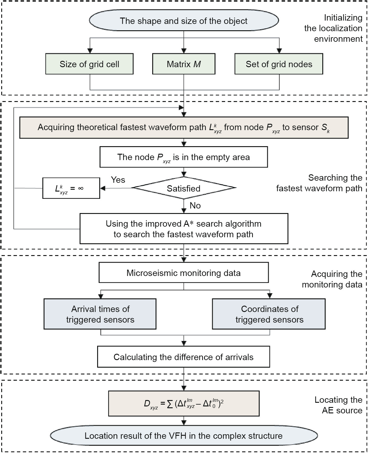
Fig. 1. The flowchart for the locating process of the VFH. S_k: the kth sensor receiving the signal; D_xyz: the deviation degree of the point P_xyz from the unknown MS/AE source P₀; : the actual time difference of the two different sensors S_l and S_m; : the travel time difference between two different stations l and m.

《2.1. Determine the initial environment》

2.1. Determine the initial environment

The geometry and specific location of the empty area is determined in the location area. Moreover, the size of the unit square grid is determined according to the condition of the empty area and the accuracy requirement of the position. In general, the denser the grid is, the higher the location accuracy is, while the calculation will be multiplied. However, the location accuracy would not be obviously improved by partitioning when the grid is sufficiently densely divided. A zero matrix M with the same size as the grid node is established, and the matrix index position ( x, y, z ) corresponding to the grid node is marked as 1. The mesh nodes form a set that serves as the starting point to search for the fastest waveform path among subsequent nodes. Assuming that the propagation velocity of the P wave in the surrounding non-empty area is a fixed unknown value and is represented by C. For the unknown source P₀, set its position coordinate to (x₀, y₀, z₀₎ , and the initial time of excitation to t₀.

2.2.1. A* search algorithm

The A* search algorithm was proposed by Peter Hart, Nils Nilsson, and Bertram Raphael of the Stanford Institute (now SRI International) in 1968 [31,32]. In computer science, the A* search algorithm, as an extension of the Dijkstra algorithm, is widely used for path finding and graph traversal because of its high efficiency. A* search algorithm achieves better performance by using heuristics to guide its search. In each iteration of its main loop, A* search algorithm picks the node based on the on the function which is consisted by two functions and . Specifically, A* search algorithm selects the path node with the minimum value at each step.

where n denotes the current node of the selected path; is used to calculate the distance of the exact fastest path from the starting node to node m ; is a heuristic function, which can be used to estimate the minimum distance from node n to the target [33]. In this paper, the Euclidean distance between two nodes is taken as the estimated minimum distance. The A* search algorithm stops searching when it expands from the starting point to the target point or when no path can be expanded.

In the actual three-dimensional application, the traditional A* search algorithm adopts the center point to search the path, and generally only 26 nodes of the adjacent layer are considered to select the next node, as shown in Figs. 2(a) and (b). In the "L” type area, the shortest path is traced by using the conventional A* search algorithm, and the path searched is shown in Fig. 2(c). It can be found from the figure that there are two unreasonable places in tracing the shortest path. ① The path obtained has a sharp jagged shape. It is caused by the limitations of the traditional A* search algorithm. ② The nodes of the path are the center of the grid, which means that the sensor should also be placed in the center of the grid, which is not applicable in the real application.

《Fig. 2》

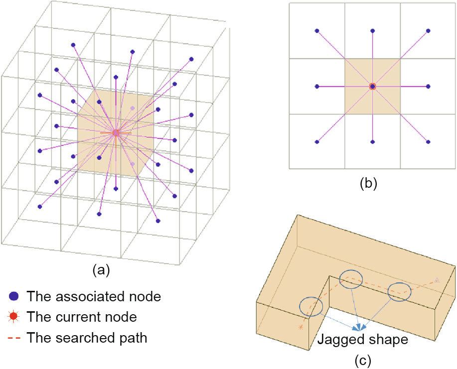
Fig. 2. The traditional A* search algorithm. (a) The current node is connected to the associated 26 nodes; (b) the main view of the Fig. 2(a); (c) the path searched by the traditional A* search algorithm.

2.2.2. Improved A* search algorithm

To trace the shortest path more effectively, the A* search algorithm is improved to search by grid points, as shown in Fig. 3. This allows the nodes of the searched path to be on the mesh node, which also means that the sensor can be attached to the surface node of the object. It is more in line with the actual situation.

《Fig. 3》

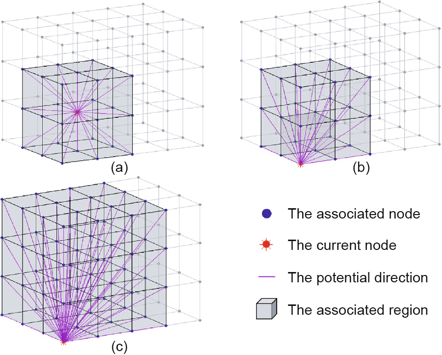
Fig. 3. The potential direction between the current grid node and the associated grid nodes. (a) The current node is connected to the adjacent one layer; (b) the current node is connected to the adjacent two layers; (c) the current node is connected to the adjacent three layers.

To avoid a sharp jagged shape of the searched path, an effective connection between the node and nodes around it is established. In the traditional A* search algorithm, one node expands to 26 nodes in an adjacent layer, as shown in Fig. 3(a). This means that the current node can only expand around 26 directions.

The more nodes in adjacent layers connected with the current node, the more directions available for the path node to select, which leads to the increasing accuracy of the searched path. Because of the symmetry of the directions between the nodes, only one eighth of the total number of directions is drawn for explanation. Figs. 3(b) and (c) shows the grid is connected to the surrounding two layers (124 nodes) and three layers (342 nodes). The relationship between the number of the node and the number of layers i is expressed as

In the process of outward expansion, certain directions formed by nodes are repeated, so it can be ignored. The computation cost can be reduced by removing these grid points. To reduce the error of the search, the amount of calculation is increased to provide more connections for each grid node.

The block model and strip model which have been meshed, are used to explore the reasonable value of layer i , as shown in Fig. 4. Suppose the source is excited at point O, and the wave reaches point K (K = A, B, C, D, E, F, G, H, A' , B' , C' , D' , E' , F' , G' , H' ) from point O, forming the path L_K . According to the geometrical relation, recording the actual fastest path distance D_R of the wave into Table 1. The path L_K is traced by using the model of the i layer (i = 1, 2, 3, 4, 5, 6,...), respectively. The relative error E between the searched path distances D_Si and D_R can be expressed as

《Fig. 4》

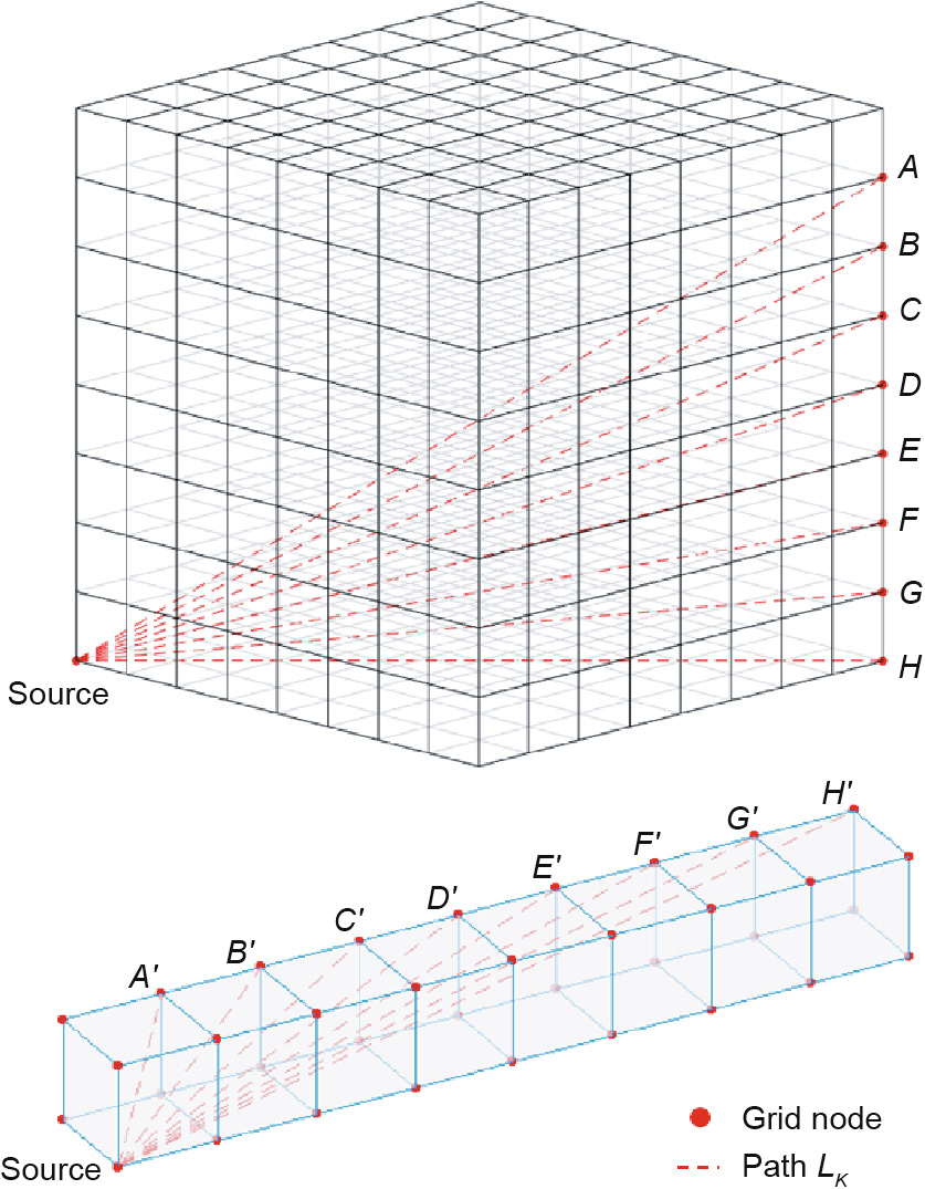
Fig. 4. The ideal paths from the source node to neighbor nodes K (K = A, B, … , H' ).

The relative error E of obtained path is recorded in Table 1, and the maximum path error E_i-_max of each model is selected. The time complexity O of the improved A* search algorithm is positively related to the number of expanded nodes Z, i.e. . Thus, the number of nodes Z can be used to approximate the calculation amount O. Fig. 5 shows the relationship between the number of layers i and E_i-_max and the number of associated nodes , respectively.

《Fig. 5》

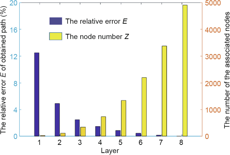
Fig. 5. The number of layers, relative errors, and the number of the associated nodes.

《Table 1》

Table 1 Relative error between the distance of actual path and the distance of searched path.

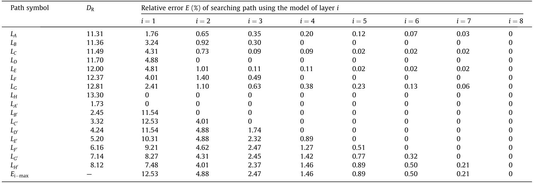
Through different testing, we found that the relative error of the theoretical path is less than 3%, when the layer number of topologies reaches 3. The relative error is influenced by the size of sensors or the system error. This means the algorithm can basically meet the location requirement with relatively small growth rate of calculation amount. Therefore, this article would utilize the A* search algorithm to establish connection between a node and the surrounding three layers. In order to determine the specific location of the path, after determining the length of the shortest path by A* search algorithm (or the Dijkstra algorithm), a reverse search is also needed. Therefore, this article adds the function of recording the coordinates of the previous node at the corresponding position of the current node when searching for a path. This is also helping avoiding reverse search and enhancing computational efficiency.

《2.3. Collect data of arrivals》

2.3. Collect data of arrivals

m sensors are installed at different positions of the specimen to capture the arrivals of the MS/AE. Each sensor is located on a grid point so the location is known. For the three-dimensional model, there are five unknowns (wave velocity of P wave, coordinates of MS/AE source (x₀, y₀, z₀) , initial time of excitation t₀), so sensor number m should be an integer greater than or equal to 5. For the kth sensor S_k receiving the signal, the coordinates are recorded as (x_k, y_k, z_k) , and the first arrival time of the received P wave signal is . Calculate the actual time difference of the two different sensors S_land S_m, denoted by .

《2.4. Source location》

2.4. Source location

For the source generated by the point P_xyz, the theoretical travel time corresponds to the shortest propagation path between the source and the kth sensor divided by the velocity C. The time difference between two different stations l and m corresponds to the difference in travel time .

According to the square of the difference between and is introduced to describe the deviation degree of the point P_xyz from the unknown MS/AE source P₀ , which is expressed as

Among them, when the sources fall into the empty area, .

Each grid point will get the corresponding D_xyz value. The deviation degree of the point P_xyz from the unknown source P₀increases with the growth of the value of D_xyz . Therefore, the coordinate corresponding to the minimum D_xyz value can be considered as the coordinate of the MS/AE source location.

《3. Results and discussions》

3. Results and discussions

The lead-breaking test was carried out on the hollow column mortar structures to evaluate the performance of the proposed method. A cubic concrete test specimen with the size of 10 cm × 10 cm × 10 cm was cut out into a cylindrical empty space with the size of 6 cm × 10 cm, as shown in Fig. 6(a). There are 10⁶cubic grid blocks of the same size to form the model when the sides of cube are 1 mm in length. To speed up the calculation, the test piece is divided into 25 × 25 × 25 cube with the size of 4 mm in length, as shown in Fig. 6(b).

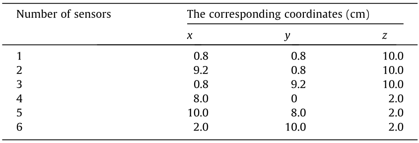
The cubes of the empty area are marked as not passed, and the other cubes as pass. Six MS/AE sensors were attached to the test piece, and a coupling agent was added between the sensor and the test piece for better acoustic coupling. The position of the sensor is located on the grid node (Fig. 6(c)), and the coordinate position is shown in Table 2.

《Fig. 6》

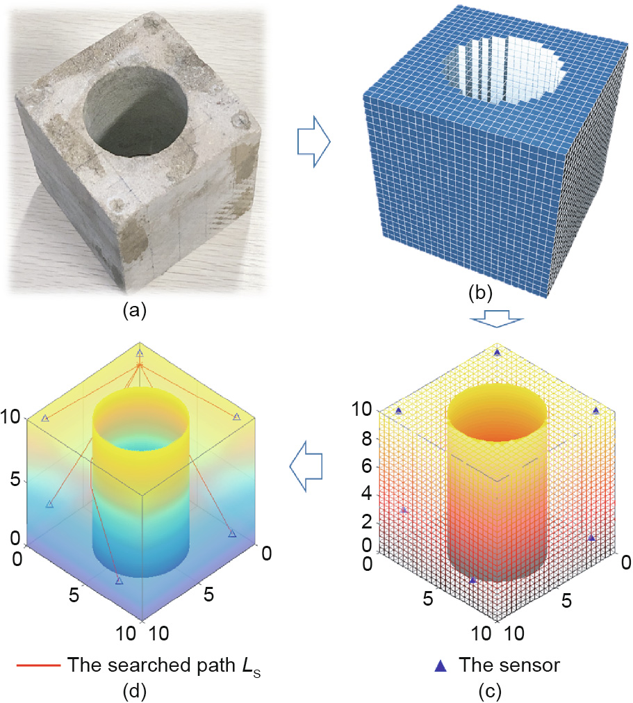
Fig. 6. The process of localization with the VFH. (a) The specimen; (b) modeling and meshing the specimen; (c) determining the coordinate of sensors (unit: cm); (d) the path searched by the improved A* search algorithm from node to sensor (unit: cm).

《Table 2》

Table 2 The coordinates of the sensors.

To facilitate the calculation, the model coordinates were transformed so that the index of the node matrix M is in oneto-one correspondence with the coordinate positions. The data acquisition uses a 40 dB threshold and a 5 MHz sampling rate. The lead-breaking tests were carried out at different positions of the test piece, and each position (shown in Appendix A Table S1) was performed twice. The arrivals of the P wave generated by MS/AE event are recorded by the sensors (Table S1). Searching the path L_S between each potential source and the sensor and calculating the distance of the path, are shown in Fig. 6(d). Then, according to the arrivals recorded by the sensors, the deviation value D_xyz of each potential source is calculated. The coordinates (x, y, z) of source location on the specimen corresponding to the minimum D_xyz is determined and is converted to the position coordinates. The location results of VFH are shown in Table 3. Meanwhile, the results of TD are performed and shown in Table 3.

《Table 3》

Table 3 Location result and error of the lead-breaking points.

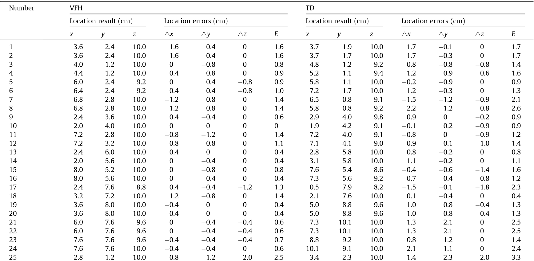
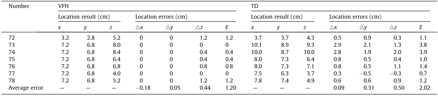
The localization results between VFH and TD with the actual lead-breaking points, and the error records are shown in Table 3. As seen from the table, the maximum location error of the TD is 4.5 cm, which is much larger than the location error of the VFH. For the convenience of observation, Fig. 7 shows the visualization of the location results and location errors of the two methods In Fig. 7(a), the circle size represents the magnitude of the error of the source localization result. It can be clearly seen that the circle of the TD is much larger than that of the VFH. Fig. 7(b) represents a boxplot of the location error E of the two methods. On each box, the central mark, the bottom edge of the box, and top edge of the box indicate the median, the 25th percentile, and the 75th percentile, respectively. The whiskers above and below the box show the most extreme data points, and the outliers are plotted individually using the "+” symbol. As shown in Fig. 7(b), the median source location error obtained by using VFH is approximately 1.0 cm, while the median location error obtained by using TD is approximately 1.9 cm. Obviously, the location results of VFH are better. Other parameters of Fig. 7(b) can also validate this view. According to the location error of each lead-breaking test in the table, the average location error of the VFH is 1.20 cm, while the average location error of the TD is 2.02 cm. The average location accuracy of the VFH is nearly 40% greater than the TD. Therefore, in the complex three-dimensional structure, the location accuracy of the VFH is greatly improved comparing to the TD.

《Fig. 7》

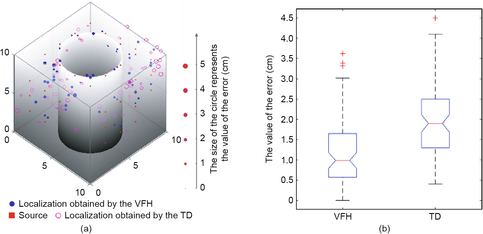
Fig. 7. Location result and error of AE sources obtained by two methods. (a) The visualization of the result and error; (b) the boxplot of the location error.

《4. Conclusions》

4. Conclusions

In this paper, a localization method without using premeasured velocity based on the A* search algorithm is proposed. It avoids manual repetitive training by using equidistant grid points to search the path. For three-dimensional complex structures with irregular spaces, the A* search algorithm is improved and grid points are used to search for paths reflecting the actual propagation of elastic waves. Moreover, the wave velocity of the elastic wave is considered as an unknown in the calculation to reduce the location error caused by the wave velocity change during the monitoring process.

To evaluate the quasi-determination and effectiveness of the VFH, a lead-breaking test was carried out on hollow cubic concrete structures. The location results show that the average location error obtained by the VFH is 1.20 cm, and its average positioning accuracy is 40% higher than the TD. It can be conduced that the proposed method in the paper can effectively adapt to geometrically irregular three-dimensional complex structures.

The VFH overcomes the disadvantages of the existing localization method, which considers the impact of geometry, and is suitable for three-dimensional hole-containing structure. The method in this paper is also applicable to other fields such as nondestructive testing of acoustic emission positioning.

《Acknowledgements》

Acknowledgements

The authors wish to acknowledge financial support from the National Natural Science Foundation of China (51822407 and 51774327), Natural Science Foundation of Hunan Province in China (2018JJ1037), and Innovation Driven project of Central South University (2020CX014).

《Compliance with ethics guidelines》

Compliance with ethics guidelines

Longjun Dong, Qingchun Hu, Xiaojie Tong, and Youfang Liu declare that they have no conflict of interest or financial conflicts to disclose.

《Appendix A. Supplementary data》

Appendix A. Supplementary data

Supplementary data to this article can be found online at https://doi.org/10.1016/j.eng.2019.12.016.

Show More