

《1. Introduction》
1. Introduction
In a global supply chain, controlling material flow from suppliers through to the final customer is a serious challenge. Firms sourcing from the global market inherit more uncertainty compared to those sourcing from the local market. Longer procurement lead times are less reliable and result in more tied up capital in the form of pipeline inventory. Bottlenecks are evident and an inherent part of every supply chain. One such bottleneck related to inventory management is imperfect quality items received from the suppliers. According to the Supply Chain Council, a perfectly fulfilled order is one with the right item delivered to the right location, at the right date and time, in defect-free condition, damage-free, in the right amount, and with error-free documentation. Naturally, it is impossible for the suppliers to provide 100% perfect quality items; a probable margin of error always remains. Upon stock taking, the buyer must check the quality of the entire lot and sort out imperfect quality items. For imported products, it is neither feasible nor economical to return defective quality items to a supplier located thousands of miles away. Imperfect quality items are sent to the in-house repair shop or to the local market for reparation and are partially backordered after being reworked.
Supply chain stakeholders coordinate and integrate their business processes to deliver superior customer value at the lowest possible cost. Traditional inventory models assume that payment is made instantly after the shipment is dispatched by the supplier or received by the customer. In reality, trade credit is advanced by the buyer on deferred payment to the supplier, namely, until after the goods are sold by the buyer. Trade credit is the allowable delay in payment for a duration of time between purchasing and settling the amount mutually agreed on by buyer and supplier. Payment terms are governed by product service agreements between the two parties without interrupting the material flow. Trade credit is a win–win strategy for supply chain partners. Generally, trade credit is offered to a lower-level partner, such as the buyer, by a higher-level partner, such as the supplier, in the supply chain hierarchy [1]. The buyer is better off with an opportunity gain (interest earned) whereas the supplier is worse off with an opportunity cost (interest paid), calculated using selling price and purchasing cost, respectively [2]. In addition to the opportunity gain due to delay in settlement of payment, the buyer continues selling items, thus getting paid by the customers but not paying back to the supplier [3]. On the other hand, the supplier views trade credit as a competitive strategy to maximize sales and minimize on-hand inventory. For the supplier, there is a tradeoff between opportunity cost and financial gain. Inventory management is all about managing tradeoffs between conflicting goals. Trade credit is a very successful strategy whereby businesses maximize their sales and, in turn, profits. Opportunity cost and opportunity gain are incorporated into the model for profit calculation.
Inventory models are built around various assumptions irrespective of their practical implications. Ahmed and Sarkar [4] stated that the management of goods from an initial source to an end customer with perfect quality is a fundamental part of a supply chain. One such assumption is that all items received in a lot are of perfect quality. Today, businesses want certainty of supply, quality, and safety [5]. The next generation of manufacturing holds the promise of increased elasticity in production, along with mass customization, better quality, and improved productivity [6]. Khanna et al. [7] proposed an optimal replenishment inventory policy for imperfect quality products. Due to the occurrence of defectives in the system, all pieces go through a 100% inspection process. According to Tiwari et al. [8], the green production system and the rework process are often imperfect. In addition, payment to the supplier is made instantly after the items are received by the buyer. Researchers have criticized such an impractical assumption and have urged inventory models to be based on realistic parameters [3]. The proposed model relaxes these assumptions to find an optimal solution to the real-life problems. The model expands on identification of imperfect quality items, reparation of these items, partial backordering after rework, and multi-trade credit policies. An algorithm, based on the algebraic approach, is developed to solve the profit maximization objective [3]. This methodology provides a closed-loop optimal solution for the objective. The algebraic approach explains the inventory theory in the best and simplest way while simultaneously minimizing the probability of error.
This paper aims to measure the effect of reworking the imperfect quality items and partially backordering those items into the system of material flow and profit. Moreover, the effect of multitrade credit on profit is assessed. This work provides practical insights to managers of home appliance supply chains, such as electrical appliances. Usually these companies source stock from overseas suppliers against an anticipated demand and any excess demand is backordered. However, returning or exchanging the damaged items is not an economical option. The subsequent sections are organized as follows: Section 2 consists of a literature review; Section 3 describes the problem definition and assumptions of the proposed mathematical model; Section 4 formulates the mathematical model; Section 5 validates the model with a numerical example and results; Section 6 details the sensitivity analysis of the proposed model; Section 7 provides managerial insights; and Section 8 concludes with a discussion of future extensions.
《2. Literature review》
2. Literature review
Modern inventory models are based on the classical model of economic order quantity (EOQ) given by Harris [9]. This model is used to determine optimal order size based on certain assumptions. Several researchers in the domain of inventory management criticize the impractical and unrealistic nature of these assumptions [3,10]. Goyal [11] relaxed the assumption of instant payment by introducing an inventory model under permissible delayed payment to the supplier. Porteus [12] argued that while producing in batches the process can go ‘‘out of control,” thus introducing the possibility of defective items. Rosenblatt and Lee [13] found a significant relationship between product quality and batch size; they maintained that reducing batch size decreases the probability of defective units. Salameh and Jaber [14] viewed that the defective products must be reused after being reworked as they are still valuable. They extended the economic production quantity (EPQ) model for defective items by taking a random sample of defective items from a batch. Roy et al. [15] extended the literature on inventory models by studying defective quality and stock-out conditions during a screening of the total lot. Stock-out can occur due to defective features, therefore, a fraction of demand is fulfilled with partial backordering.
The literature on production and inventory models has evolved overtime. Various researchers have extended the debate by relaxing inventory model assumptions and integrating multiple dimensions of inventory management, thereby making it more applicable. Eroglu and Ozdemir [16] introduced an extended inventory model whereby they assumed that each inspected batch has defective items, and the shortages were backordered. Later, Sarkar et al. [17] put forward a single stage economic production model considering random defect rate for imperfect quality items. The model introduced a process to rework or repair defective quality items with anticipated backorders. Sarkar and Saren [18] introduced a model that assumed a screening policy, number of screening errors, and guarantee costs for non-screened items. They found that in the case of 100% inspection, the screening cost significantly adds to the cost of inventory. Jaber et al. [19] extended the inventory model by substituting defective quality items with contingent local emergency purchases, which were at a higher cost. Lashgari et al. [20] introduced an inventory model with downstream partially delayed payment and up-stream partial prepayment under three scenarios: without shortage, with full backordering, and with partial backordering. Sarkar et al. [21] put forward an integrated model by using the classical optimization technique for defective quality items assuming two-stage inspection, variable transportation cost, and fixed rework cost. Ahmed and Sarkar [22] stated that a well-designed supply chain is necessary to use renewable products at a commercial scale. For that reason, it is necessary to improve and plan a supply chain that is economical. Kim and Sarkar [23] developed a multi-stage production system for cleaners to improve quality by removing all unacceptable quality items during the manufacturing procedure. They used the logarithmic expression from Porteus [12] for quality improvement in a single-stage manufacturing process with imperfect quality.
Recent studies on imperfect production and inventory models have integrated multiple facets of inventory decision making, such as environmental concerns, preventative maintenance, and uncertain demand. New opportunities in intelligent manufacturing may include defect-free production by means of opportunistic process planning and scheduling and control of complex supply chains [24]. Certainly, effective information sharing can improve production quality, reliability, resource efficiency, and the recyclability of end-of-life products [25]. However, even in the current era the production system does not supply 100% perfect items. Tiwari et al. [26] presented an inventory model for a single-vendor/singlebuyer system with defective items and carbon emissions during transportation, warehousing, and storage. Taheri-Tolgari et al. [27] studied defective items and preventative maintenance in a production system in order to establish a screening policy and optimum inventory level under uncertain conditions. Tayyab et al. [28] studied the effect of defective items and uncertain product demand in a multi-stage production model. A fuzzy theory and center of gravity approach was used to deal with demand uncertainty and to defuzzify the objective function, respectively. Wook Kang et al. [29] introduced a single-stage manufacturing model with screening, defective items, rework, and planned backorders. The analytical approach was used to find the optimal batch size and anticipate backorders. Dey et al. [30] developed a model for a two-echelon production system to reduce defect rate and setup cost through investment.
Supply chain partners collaborate in their business operations to gain or sustain competitive advantage in the global marketplace. Trade credit policy has become an international best practice and a win–win situation to sustain partnerships. Various authors have extended inventory models by relaxing the assumption of instant payment and estimating the resulting impact on inventory management, sales, and profits. For example, Soni and Shah [31] formulated an optimal ordering strategy for retailers with demand partially constant and partially dependent on stock, and the supplier advancing multi-period trade credit. Sarkar et al. [32] discussed the sustainability issues with multi-level trade credit and a single-setup-multiple-delivery policy. Their model improves the economic and environmental performance of three-echelon supply chains. Yang and Tseng [33] introduced an inventory model to maximize the profit of a multi-echelon supply chain with permissible trade credit and backordering under controllable lead times. Recent studies have advanced the literature on inventory models to next level by measuring the impact of multiple practices including imperfect quality, backordering, rework, trade credit, and multi-trade credit periods. For example, Taleizadeh et al. [34] advanced the inventory model by studying the effect of defective items, upstream and downstream trade credits, and backordered demand. Tiwari et al. [35] identified the potential circumstances that may take place in inventory models under different allowable delay-in-payments. Mohanty et al. [1] introduced an integrated buyer–supplier inventory system with defective items and trade credit in order to reduce set up cost and shortages. Taleizadeh et al. [36] developed a single-machine manufacturing system for multiple products with the assumptions of defective items and trade credit. In particular, the model is designed to obtain the global optimum in terms of cycle length, production quantity, and backorder quantity of each product such that the total cost is minimized. Tiwari et al. [8] and Lashgari et al. [37] developed an ordering policy for non-instantaneously deteriorating items with multiple advances and a delayed payment schedule. Zia and Taleizadeh [38] further enrich the EOQ model by integrating backordering with a hybrid payment scheme linked with order quantity to stimulate sales. Lashgari et al. [39] developed an inventory control model for perishable items in order to study the impact of trade credit linked with order quantity over a finite time. Table 1 summarizes the contribution of different authors and compares them against the proposed model [1,11–21,23,26–31,33,34,36–43].
《Table 1》
Table 1 Typology and review of inventory models.

Taleizadeh et al. [43] developed an inventory model for imperfect items with partial backordering. They considered three scenarios at the time of receipt of the backordered items: first, received exactly when the inventory level is equal to zero; second, received when the backordered quantity is equal to the imperfect items; and third, received when the shortage remains. Taleizadeh et al. [44] further extended the inventory model by considering a fourth scenario where the backordered items are received when the inventory level is in excess. Sarkar et al. [3] and Ahmad et al. [45] studied the second and fourth scenarios, respectively, as identified by Taleizadeh et al. [44] under the multi-trade credit period. Taleizadeh et al. [46] developed an EOQ model with probabilistic replenishment intervals and permissible delay-in-payments with partial backordering. Taleizadeh et al. [43] introduced three different imperfect item replenishment scenarios under partial backordering and studied their individual impact on cost minimization. No system is perfect, therefore a certain percentage of lot items will be imperfect. This problem becomes more critical when the supplier is located far from the buyer, such as in global supply chains. This study aims to measure the impact of the third scenario on profit under multi-period delay-in-payments.
《3. Problem description and assumptions》
3. Problem description and assumptions
This part of the study draws the problem description and assumptions of the developed research.
《3.1. Problem definition》
3.1. Problem definition
In the global supply chain, the purchaser manages to buy goods from a supplier located miles away. It is next to impossible for 100% of the items to be perfect. It is also possible for items to have inbuilt defects from the production process. Similarly, damage can be caused by mishandling during the global transport process. During the stock taking process the buyer screens out some percentage of imperfect quality items. It is presumed that the defective quality items can be repaired at a local reparation shop. Returning these items to the overseas supplier, located thousands of miles away, for exchange is neither feasible nor economical. After repair, the now-perfect items are partially backordered into the initial inventory. It is noteworthy here that the cost of holding original inventory is less than reworked items. The repair cost entails two major cost heads, variable cost and fixed cost. The variable cost consists of unit transportation cost per defective item, raw-material cost, worker expense per defective item, and holding cost for the reworked items at near-by repair store. The fixed cost consists of the setup cost for the local store and transport costs. The time reworked items add to the initial inventory has a significant impact on stock and, as a result, the customer service level. In this study, the assumption is made that reworked items re-enter the purchaser’s inventory as stock shortages occur and the quantity of reworked items is equal to the shortage. Moreover, it is assumed that the buyer has been allowed a multi-period delay-inpayment policy by the supplier. In other words, the buyer benefits from a varying level of opportunity gain over multiple periods. There is a need to design an efficient inventory management model that can maximize profit by optimizing the lot size (Q) with an optimal portion of cycle time (F) and a cycle time (T) by integrating multi-period delay-in-payment and partial backordering. The inventory structure for rework of defective quality products is shown in Fig. 1.
《Fig. 1》
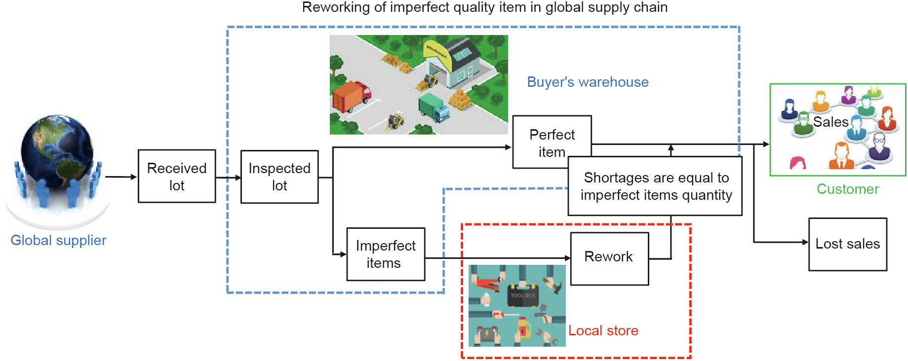
Fig. 1. Flow of inventory system for reworking items with defective quality.
《3.2. Assumptions》
3.2. Assumptions
The mathematical model is structured on the following assumptions:
(1) The structure has a singular item.
(2) Received consignment may contain defective items.
(3) The systems allow shortages, which are partially fulfilled.
(4) The buyer receives the lot from the global supplier, and the cost of sending defective items back to the global supplier is more expensive than repairing the items at a local repair store.
(5) Screening and demand rates are taken as known and constant.
(6) The demand fulfillment and inspection process take place in parallel, but the inspection rate is more rapid than the rate of demand (x>D).
(7) Imperfect items have minor defects and can be reworked at a local store.
(8) The percentage of defective items is known and given.
(9) The correlation between cost of procuring Cu by buyer and price of selling P by buyer is given by P ≥ Cu.
(10) The repaired items have holding costs greater than the original holding cost of undamaged items (hr > h).
(11) The reworked items are reverted as soon as shortages are equal to the quantity of imperfect items.
《4. Mathematical modeling》
4. Mathematical modeling
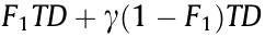
This section develops and explains an assimilated inventory model of total profit with partial backordering, reparation of imperfect items, and multi-delay-in-payments, as shown in Fig. 2. The inventory level remains positive during F fraction of time. It is equal to F1 + F2. These are taken as F1 = ( 1– β) F and F2 = βF, where β is the proportion of imperfect items. The positive inventory level of the system is taken as FT, where T is the cycle time. The Fi ( i = 1, 2) is within a [0, 1] interval. If F is equivalent to zero, then loss of all demand will occur, whereas if F is equal to exactly one shortages do not occur. The proposed state inventory level is FTD. The initial batch is inspected at rate x during inspection time ts= FTD/x. The screening rate is faster than the demand rate (x > D). After screening period ts, the β percentage of items with imperfect quality (βFTD) are carried out of inventory and transported to a rework shop. The reworked items are carried back to the buyer’s warehouse after interval tR. The tR is an accumulative period of transport and rework time. The rework activity at the local shop follows controlled coordination. The fixed cost of the repair store is sr + 2A, where sr is the setup expense of the local store and A is the fixed cost of transportation. The variable cost is given by clm + 2ct + hstR for imperfect items, where clm is employment and material cost, ct is transport cost, hs is holding cost at the repair store, and tR is the aggregate repair duration which consists of transport, coming back, and reparation duration of defective pieces. The repair period is given by tR = tT + βFTD/R. The complete cost for the local store is given as sr + 2A + βFTD ( clm + 2ct + hstR) . If hr is the holding cost of the repaired products and h is the initial unit holding cost then h < hr. As repaired items are being reworked shortages are occurring in the inventory system. It is assumed that the reworked items come to the inventory system when the shortage level is equal to the quantity of repaired items. Ultimately, the inventory level becomes equal to zero. In the proposed case, the order quantity per cycle is given by Q = F1TD +  =
= when shortages are equal to the quantity of imperfect items, where
  is the proportion of demand that is backordered.
《Fig. 2》
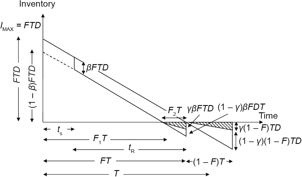
Fig. 2. Status of defective item inventory and the arrival of reworked items. IMAX: maximum inventory level.
《4.1. Cost of ordering》
4.1. Cost of ordering
In individual cycle T, the buyer suffers a single period cost of ordering, which is denoted by OC, where O is the fixed cost of ordering and presented as

《4.2. Screening cost》
4.2. Screening cost
The screening cost of an entire batch is represented by SrC, which is presented by

where the inspection cost of one unit is given by Cs, F is the length of inventory with a positive period, and D is the demand rate.
《4.3. Holding cost》
4.3. Holding cost
The aggregate of the holding cost of perfect goods and the holding cost of repaired products results in the total holding cost HC, which is written as

《4.4. Repairing cost》
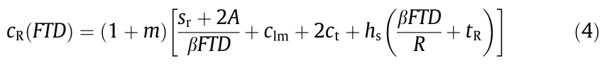
4.4. Repairing cost
If m margin is the repair charge per unit, then repairing cost, cR, for one unit is expressed as
The arrival of reworked items occurs when shortages are equal to the quantity of imperfect items, consequently, inventory is then βFTD units. As the cycle finishes, (1– F )TD becomes shortage level of the system. For a given cycle, the quantity ordered is denoted as Q = FTD + 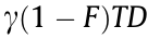 .
.
《4.5. Shortage cost》
4.5. Shortage cost
The shortage cost SC is given by the following notation:

where π is the backordered cost,  is the cost of lost sales, and
  is the percentage of backordered demand.
《4.6. Goodwill penalty cost》
4.6. Goodwill penalty cost
The goodwill penalty cost GWC is taken as

where w is the percentage of imperfect items delivered to customers, v is the return cost of manufactured goods, and g is penalty cost due to loss in goodwill.
《4.7. Interest charged and interest income earned》
4.7. Interest charged and interest income earned
In the permissible delay-in-payment strategy, if payment time is higher than lead time, the buyer earns additional interest income. If the permitted time is less than the lead time, then the buyer earns less interest income and pays more in opportunity cost while the supplier gains interest income and pays less in opportunity cost. As a result, the supplier’s model has two succeeding cases, established by the permitted time of payment and the length of lead time. The difference in cost concerning those two expected cases are as follows.
Situation 1: If lead time T is equal to or less than the allowable payment period M, then only interest income is earned because interest charged in this condition is zero. This condition is presented in Fig. 3, and can be written as

where P is the sales price, Ie is the interest earned.
《Fig. 3》
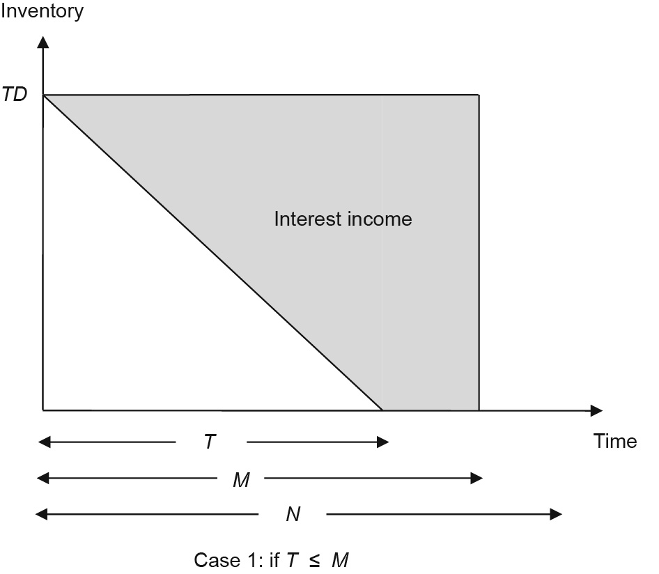
Fig. 3. Graphical demonstration of interest when T ≤ M.
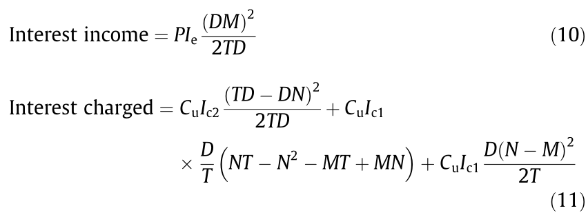
Situation 2: If the lead time T is greater than the initial allowable payment time M, and equal to or less than the subsequent allowable payment time N, then interest cost is charged as well as earned. This condition is presented in Fig. 4, and can be written as

where Ic is the interest charged.
《Fig. 4》
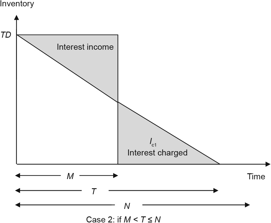
Fig. 4. Graphical demonstration of interest when M < T ≤ N.
Situation 3: There is also a special case where extra interest is charged to the buyer if they fail to give the required payment in the initial allowed time. In this case, lead time T is greater than the subsequent allowable payment time N. This condition is presented in Fig. 5, and is given as
《Fig. 5》

Fig. 5. Graphical demonstration of interest when T > N > M.
Total profit function: Total profit = Selling price – (Ordering cost + Product cost + Screening cost + Holding cost + Rework cost + Shortage cost + Goodwill penalty cost + Interest earned + Interest charged)
Under the above mentioned situations of multi-period delay-in-payments, three cases are established and the total profit equation for these three cases are formulated as:
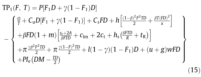
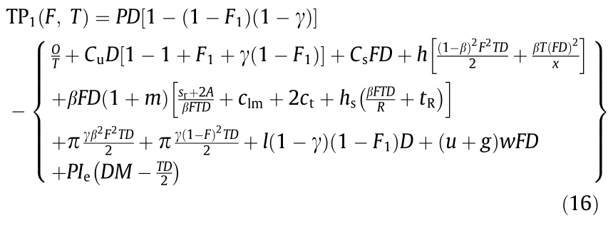
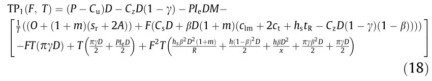
Case 1: The equation of total profit (TP) will be a combination of Eqs. (1)–(6) and Eq. (7), in which lead time T is equal to or less than the allowable payment period M, resulting in earned interest income and zero interest charged, that is TP1 if T ≤ M,

where u is the refunded cost of the defective item.
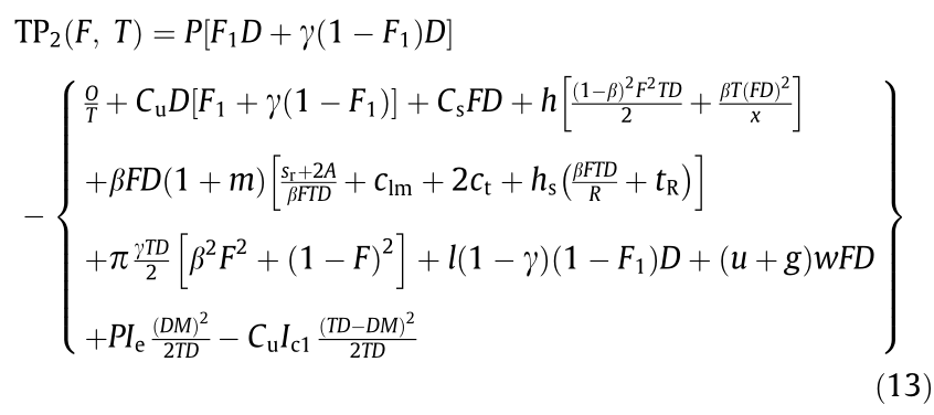
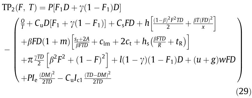
Case 2: The equation of total profit will be a combination of Eqs. (1)–(6) and Eqs. (8) and (9), in which lead time T is greater than the initial allowable payment time M, and equal to or less than the subsequent allowable payment time N, resulting in interest costs being charged as well as earned, that is, TP2 if M < T ≤ N,
Case 3: The equation of total profit will be a combination of Eqs. (1)–(6) and Eqs. (10) and (11), in which extra interest is charged to the buyer if they fail to give the required payment during the initial allowed time, that is, TP3 if T > N > M,

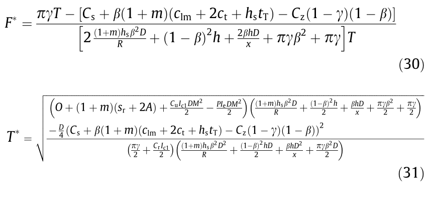
《4.8. Case 1 with optimal values of T and F》
4.8. Case 1 with optimal values of T and F
The profit equation according to Eq. (12) for Case 1 can be formulated as
Therefore, it is noted that 
 , thus, the profit function can be expressed as

By putting  , the total profit function becomes

Additionally, the function can be streamlined as
with  as constant terms. If the total cost is minimized, then the total profit is maximized. Also, if
 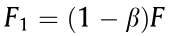 is considered, Y(T, F ) is written as
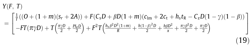
The compressed formula of Y(T, F ) can be expressed as

For values of J1 –J5 see Appendix A Section 1.
Eq. (20) is re-written as

where  .
.
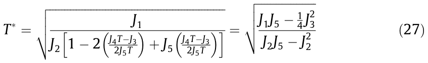
The cost equation has the least value with respect to T when (see Ref. [15] for detail)
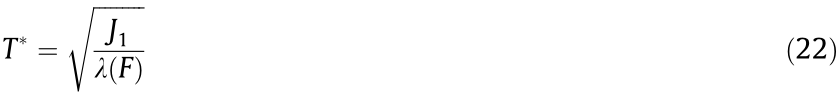
The total cost is the lowest possible if we substitute T* in the cost function

The optimal value of T can be subject to F. A non-derivative methodology is applied to develop the optimal values of F. The developed structure of equations proceeds only the portion of the function that entails the decision variables, and is given as
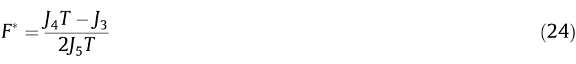
As a result of placing J4, J3, and J5 in Eq. (24):
From Eq. (22)

Placing the optimal F value in Eq. (26):
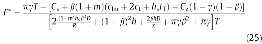
Then, finally, by placing J4, J3, and J5 in Eq. (24):

《4.9. Case 2 with optimal values of T and F》
4.9. Case 2 with optimal values of T and F
The profit equation according to Eq. (13) for Case 2 can be formulated as
The F* and T* having optimum values of (see Appendix A Section 2)
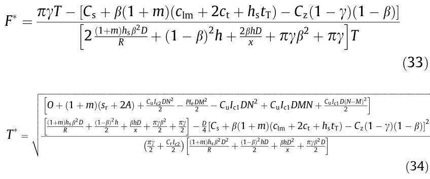
《4.10. Case 3 with optimal values of T and F》
4.10. Case 3 with optimal values of T and F
The profit equation for Case 3, as per Eq. (14), with the addition of +1 and –1 in order quantity, can be formed as

The F* and T* having optimum values of (see Appendix A Section 3 for details)
《5. Numerical experiment and results》
5. Numerical experiment and results
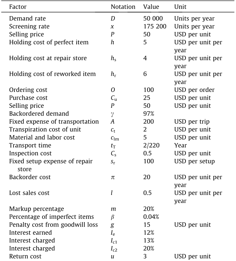
The numerical experiment is described in this section. The data for the experiment and the optimal solution for each profit and decision variable, and for each proposed case, are shown in Tables 2 and 3. The data is sourced from Taleizadeh et al. [36] with the additional parameters of lost sale, return cost, and delay-in-payments from Sarkar et al. [3]. Fig. 6 graphically demonstrates the optimum solution for various circumstances.
《Table 2》
Table 2 Numeric data for the experiment.

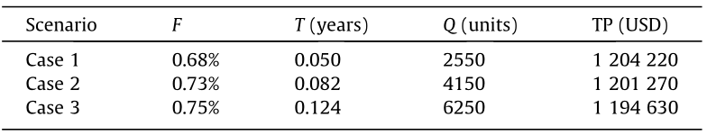
《Table 3》
Table 3 Optimal total cost for different scenarios.
《Fig. 6》

Fig. 6. Results with optimum profit for different cases.
The solution indicates that the optimum for Case 1, where total profit is 1 204 220 USD, occurs when cycle time is equal to 0.050 of a year, during which the optimistic inventory level is 0.68%, and the number of ordered units is 2550. In this case, cycle time is equal to or smaller than the first permissible payment period. For Case 2, the optimum, is attained when the cycle is 0.082 of a year, during which the optimistic inventory level is 0.73%, and the number of ordered units is 4150, which contributes a total profit of 1 201 270 USD. For this case, cycle time is greater than the first permitted payment period and smaller than or equal to the second permitted payment period. For Case 3, the optimum is attained when the cycle time is 0.124 of a year, during which the optimistic inventory level is 0.75%, the number of ordered units is 6250, and total profit is 1 194 630 USD. In this case, cycle time is greater than the first and second permitted payment periods. Clearly, Case 3 provides the greatest profit and Case 1 the least.
These results prove that profit is smaller if the permitted period given by supplier to buyer is equal to or greater than the cycle time, and profit is greater if the permitted period is smaller than the cycle time. The buyer financially benefits and makes a profit both from selling items and from earned interest. The best outcome for cycle time is obtained using certain parameters, however, an optimistic inventory level, F, is subject to change and must be in the interval of [0, 1]. If F is equivalent to zero, then loss of all demand will occur. Conversely, if F is equal to one, then shortages do not occur. As shown in Fig. 7, increases in the amount of backordered demand raises the total profit in all cases. Furthermore, it is noteworthy that the total profit is reduced by increasing unit holding costs in all cases, as shown in Fig. 8. If the unit holding cost is too high, then it is not feasible to meet the permitted period for the optimum solution. Additional investigation of total profit as a result of several fluctuating factors is displayed in the following section.
《Fig. 7》
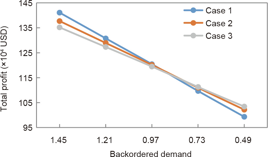
Fig. 7. Analysis of profit with different scenarios by varying the backordered demand.
《Fig. 8》
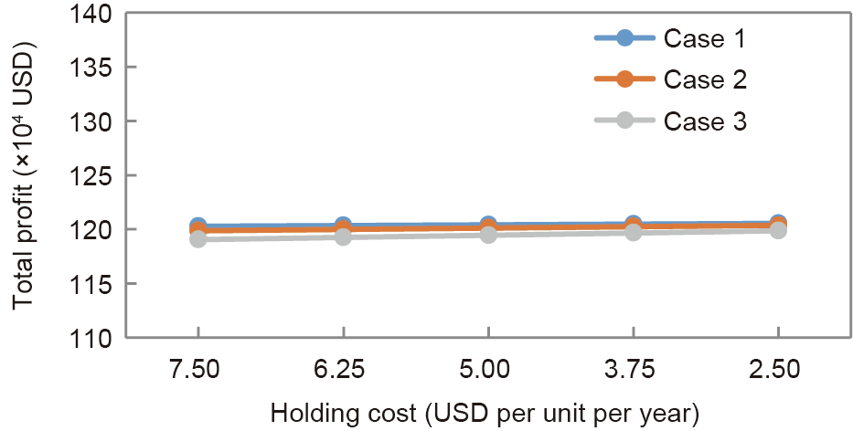
Fig. 8. Analysis of profit for different scenarios by varying the holding cost.
《6. Sensitivity analysis》
6. Sensitivity analysis
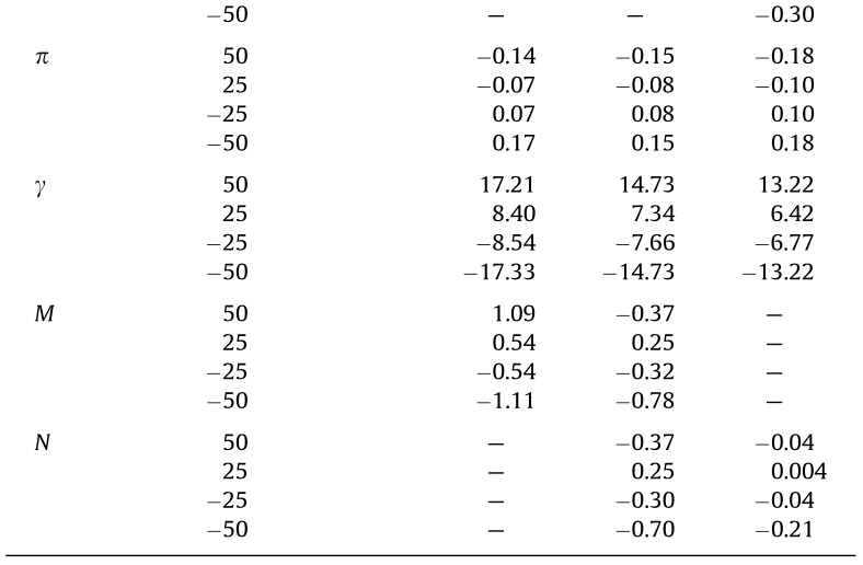
A sensitivity analysis of the effect of changes in key parameters on the total profit for cases TP(T, F )can be viewed graphically in Figs. 7–9 and in Table 4; the parameters were: holding cost h, transportation cost ct, labor and material cost for repair clm, percentage of the return of defective quality items w, interest earned per dollar per year Ie, interest charged for period one Ic1, and period two Ic2, backordered cost π, backordered demand γ, first permitted delay period M, and second permitted delay period N. The results show that a change in the value of holding cost h causes a minor inverse change in TP for each case, suggesting a state of equilibrium. The results also show that total profit is likewise sensitive to negative and positive changes in h. Similarly, the fixed transportation cost of defective items to and from repair shops ct, the material and labor cost for reparation clm, and the percent of defective items returned w, generates a small but opposite change in total profit for all three cases. The change in interest earned per dollar per year Ie results in a minor but positive change in TP for each case. The results show that TP is significantly and positively related to Ie in a state of equilibrium. The change in interest charged Ic1 is not valid for Case 1, similarly Ic2 is not valid for Case 1 or Case 2, as no interest is charged for these cases. A state of equilibrium exists in the change patterns. The change in backordered cost π results in a minor but opposite change in TP for each case. The change in backordered demand γ results in a considerable change in TP for each case. The change in the value of the first permitted delay period M results in a marginal change in TP for Case 1 and Case 2 only. Thus, this parameter does not demonstrate an equilibrium state. The change in the value of the second permitted delay period N results in a change in TP for Case 2 and Case 3 only.
《Fig. 9》
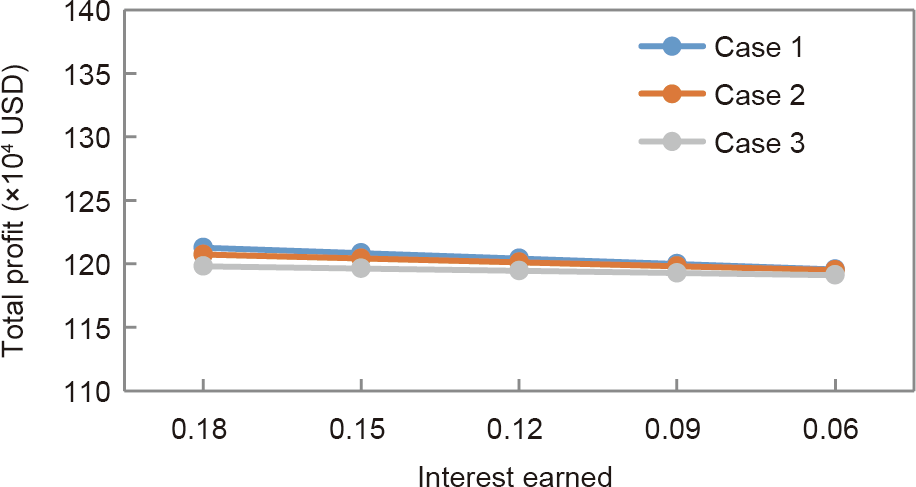
Fig. 9. Analysis of profit for different scenarios by varying interest earned.
《Table 4》
Table 4 Sensitivity analysis of the key parameters.

《7. Managerial insights》
7. Managerial insights
This study provides key insights for industrial managers under the framework of faulty-item inventory, repair of imperfect goods at a local store, and a multi-trade credit period. Total profit is maximized in scenarios where the cycle time is greater than the multiple allowable delay payment time given from suppler to buyer. Firm managers must make a decision on the fraction of the time for the optimistic level of inventory and the cycle. Therefore, a tradeoff between parameters is necessary for long lasting business payback. This study also illustrates an in-depth analysis of total profit for industrial managers by fluctuating parameters, such as partial demand of backordering, material cost for repair shops, interest paid, interest earned, unit holding cost, and transportation costs of imperfect items.
Furthermore, this research provides a path for firms to deal with unsatisfactory items if the seller is global. These flawed goods are still valuable and repairable. In order to obtain maximum profit, managers have to prioritize the acceptable delay payment period policies, cycle time, and partial backordered demand. Managers must adopt a direction to upturn sales by measuring the permissible delay-in-payment period so that it cuts the inventory of items in stock. Controlling the main parameters by systematically considering their interactions gives maximum profit. The outcome of this study provides practical implications for industry managers to attain the optimum scenario.
《8. Conclusions》
8. Conclusions
This study introduced an inventory model by integrating partial backordering and multi-delay-in-payments with an inventory structure to accommodate reparation of defective items. For this purpose, the manufacturing system of a global supplier was not perfect and produces imperfect items. Moreover, it is possible that the expected repaired batch may also contain defective items. Considering the manufacturer was far away, it was costly and timeconsuming for the purchaser to have to use reverse logistics in order to replace imperfect items. These defective goods were still valuable and needed only minor reworking in a local repair store. The proposed solution would also have a positive impact on the environment compared to sending items back to the global supplier. In this context, the proposed framework extended the existing body of knowledge on inventory models with defective goods by allowing flaws in the final product to be repaired at a local store, thus minimizing lost sales and partial backordering. After the rework, the repaired items were integrated back into the initial inventory pool. The repaired goods were reverted when the backorder demand became equal to the quantity of imperfect items received from the local repair store. The proposed model also integrated the inventory system with the best practice of trade credit in terms of multi-period delay-in-payments. This best practice will provide short term financial relief to the buyer as well as benefit the supplier by increasing sales. The optimum results with respect to diverse setups of cycle time and multi-period delay-in-payment were obtained. A non-derivative approach was employed to develop the inventory model with the objective to achieve closed-form results. This methodology was effectively used and validated in previous research. Moreover, the proposed model was established and validated with the help of a numerical experiment. Furthermore, a sensitivity analysis of key parameters was performed to support managerial decision making.
This study exploits the fundamental properties of the entire profit equation by creating a strategy with multi-period payments and employing it to mark conjectural results. Mutual understanding between companies was cast-off to develop the best profit. The research may also influence a firm’s short-term cashflow. Practitioners can increase a firm’s turnover by striking the right balance between the amount of settlement needed and the availability of resources. If the primary holding cost of non-defective items is greater than the second permitted period, then it is not feasible to get the optimal solution. This model helps to augment the performance of sustainable inventory management with a global supplier by adjusting the fraction of time with positive inventory and cycle time under multi-trade credit period partial backordering. Future research can extend these findings by testing bi-product and bi-buyer scenarios. Supplying new perfect items as a substitute for reworked items in this model is a another direction for future research.
《Compliance with ethics guidelines》
Compliance with ethics guidelines
Waqas Ahmed, Muhammad Moazzam, Biswajit Sarkar, and Saif Ur Rehman declare that they have no conflict of interest or financial conflicts to disclose.
《Nomenclature》
Nomenclature
Decision variables
T cycle time (unit time)
F section of cycle time with optimistic level of inventory (%)
Dependent variable
Q size of order in one cycle (number of unit)
Parameters
D demand (unit)
x rate of screening (unit)
ts time required for screening items (time unit)
tR transport, repair, and return time of defective items (time unit)
tT aggregate transport time of defective items (time unit)
R rate of reworking (units per time unit)
A transportation fixed cost (USD per trip)
β proportion of imperfect items (%)
O ordering cost of buyer (USD per order)
sr setup cost of rework shop (USD per setup)
h holding cost for good items (USD per unit per time unit)
hr holding cost for repaired items (USD per unit per time unit)
hs holding cost at a local store (USD per unit per time unit)
Cs cost of screening (USD per unit)
Cu cost of purchasing (USD per unit)
ct transport cost of the imperfect item (USD per unit)
clm work and material cost needed to rework an item (USD per unit)
l cost of loss of sales (USD per unit per time unit)
g penalty cost payable to loss in goodwill (USD per unit)
w proportion of defective items delivered (%)
u refunded cost of the defective item (USD per unit)
π cost of backordering (USD per unit per time unit)
P sales price (USD per unit)
γ proportion of demand that is backordered (%)
m markup fraction by local store (%)
Ie interest earned (%)
Ic1 interest charged (%)
Ic2 interest charged (%)
M 1st period for delay-in-payment (time unit)
N 2nd period for delay-in-payment (time unit)
《Appendix A. Supplementary data》
Appendix A. Supplementary data
Supplementary data to this article can be found online at https://doi.org/10.1016/j.eng.2020.07.022.


 京公网安备 11010502051620号


