

《1. Introduction》
1. Introduction
Due to the recent acceleration of industrialization and urbanization, sewage discharge is increasing in China, reaching 69.96 billion tonnes in 2017 [1]. China has made considerable efforts to decrease the impact of immense sewage discharge, for example, the construction of new wastewater treatment plants (WWTPs), expansion of the treatment capacity of WWTPs, and modification of wastewater discharge standards. At the end of 2018, a total of 5370 WWTPs were operating, with a total treatment capacity of 2.01 × 10⁸ m3 ·d–1. The overall electricity consumption reached 1.973 × 10¹⁰ kW·h [2]. The existing WWTPs continue to experience several problems such as unstable effluent, high energy consumption, and low-level automation. As one of the most widely used wastewater treatment processes, a sequencing batch reactor (SBR) has the advantages of being a simple process with a flexible operation mode, and excellent influent loading resistance [3]. However, the effluent total nitrogen (TN) concentration of this process is fluctuant, leading to unsatisfactory discharge and energy consumption. According to recent studies [4], the main reason for this problem is the low-level automation of the SBR process.
The TN removal process in the SBR is complex and includes nitrification and denitrification. Moreover, aerobic and anoxic conditions are suitable for nitrification and denitrification, respectively [5]. Dissolved oxygen (DO) is considered to be a significant factor for nitrogen removal process control. During a biological wastewater treatment process, sufficient DO is necessary to ensure the degradation and nitrification of organic matter. Excessive DO leads to high energy consumption, deterioration of sludge flocs, and lowefficiency denitrification [6]. However, the precise control of DO is rarely achieved in the biological wastewater treatment system of WWTPs, and unstable nitrogen removal occurs. According to previous studies, inaccurate monitoring and the slow response of DO caused by unmatched equipment are the main reasons for these shortcomings. In contrast, traditional simulation models and control theory are backward, and the non-timely DO data is another reason for an unstable nitrogen removal process [7,8].
In most WWTPs, engineers usually adjust the DO concentration empirically via controllable parameters such as superficial gas velocity and anoxic time. Compared with the difficulty in the precise control of DO, superficial gas velocity and anoxic time are prone to be controlled, because these parameters provide accurate regulation, precise monitoring, and a fast response. Therefore, an advanced SBR simulation model should be established with superficial gas velocity and anoxic time as the main input parameters instead of DO, and hence, the imprecise control of DO would be effectively avoided. Furthermore, the TN removal performance could be predicted more precisely.
Considering that biological wastewater treatment is a multiparameter and complex process, traditional biochemistry models are not likely to be applied at an engineering scale because of the poor learning ability for high dimensional and nonlinear data [9,10]. As an effective tool for predicting complicated nonlinear systems, artificial neural network (ANN) is gradually being developed as an appropriate method to simulate the complex biological treatment process in WWTPs. ANN is a self-learning method and has the ability to approximate any nonlinear functions [11–13]. From the perspective of neuron topology, it could be divided into the feedback neural network and feedforward neural network (FFNN), and an FFNN model could theoretically approximate any continuous function with arbitrary precision and possess the strong ability of classification and pattern recognition [14–19]. To improve the prediction ability and efficiency of an FFNN, multifarious optimization algorithms have been proposed, including Levenberg– Marquardt (L–M), Bayesian regularization (BR), scaled conjugate gradient (SCG), momentum, and Nesterov accelerated gradient. All these algorithms could significantly improve the prediction ability and efficiency of an FFNN model [20–22].
In this study, an efficient simulation model was constructed for an SBR process to achieve better prediction and control of effluent TN concentration. Compared with previous studies, the model made significant progress in two main aspects: ① The controllability of TN removal was improved by applying superficial gas velocity and anoxic time as the main input parameters instead of the regular index of DO, and ② the prediction accuracy of the simulation model was improved, based on an optimized FFNN. The objectives of this study are to ① evaluate the prediction performance of effluent TN concentration on an SBR process based on the optimized FFNN model, and ② achieve the accurate control strategy with controllable operation parameters to realize the efficient removal of pollutants and lower energy consumption at most of the WWTPs.
《2. Materials and methods》
2. Materials and methods
《2.1. Long-term simulation of SBR process》
2.1. Long-term simulation of SBR process
Two paralleled reactors (R1, R2) were established to achieve a long-term (two months) biological process simulation of an SBR process. To better simulate the actual situation of wastewater treatment, the reactors were constructed according to the SBR process in the Dingqiao WWTP in Zhejiang, China. The activated sludge in the two reactors was inoculated with seeding sludge from the Dingqiao WWTP. The synthetic wastewater was prepared according to the actual wastewater. The detailed structure of reactors and composition of synthetic wastewater are shown in Fig. S1 and Table S1 in Appendix A.
According to the actual operation mode of the SBR process at the Dingqiao WWTP, each reactor ran for four hours per cycle with a volume exchange ratio of 50%, including feeding period (5 min), anoxic and aeration period (210 min), setting period (5 min), decanting period (5 min) and idle period (15 min). For the fluctuation of actual influent wastewater quality, the concentration of major influent quality indicators was randomly controlled at 75%–125% of the preset value. Superficial gas velocity and anoxic time were set as control variables with four design values (Table 1). Following standard methods [23], the influent and effluent were sampled periodically to analyze the concentrations of TN, ammonia nitrogen (NH4+ –N), chemical oxygen demand (COD), and total phosphorous (TP). After the two-month simulation period, 124 groups of data were collected from a total of 16 combinations of control variables, with different values.
《Table 1》
Table 1 Design values of controllable operation parameters in SBR process.

To simulate more complicated condition in real SBR process, an extended experiment was constructed with a wider range of controllable variables and different influent ratio after anoxic period (Table 2). A total of 91 groups of data were collected from combinations of these variables, and 11 groups of data were collected from combinations of two superficial gas velocities (3.6 and 4.8 cm·s-1 ) and two anoxic times (0 and 150 min) to simulate the extreme condition.
《Table 2》
Table 2 Design values of controllable variables and influent ratio after anoxic period in extended experiment.

《2.2. FFNN modeling》
2.2. FFNN modeling
The base FFNN model and its optimization algorithm were built and operated in the Matlab R2016a program. Before modeling, the data set, gathered from long-term simulations, were normalized to the range of 0.001–0.999 to eliminate the effect of different dimension. A relatively ideal FFNN model was obtained by constant optimization, and its weight network was adjusted by the error between predicted and actual values (Eq. (1)) [24]. The structure of the neural network consisted of an input layer, a hidden layer, and an output layer. Six variables, including influent water quality (COD, TN, NH4+ –N, and TP) and operation parameters (superficial gas velocity and anoxic time) were set as the input of the base FFNN model, and the effluent TN was set as the output. The scheme for base FFNN modeling and coding are illustrated in Fig. 1. The dimension of experimental data was relatively low, and therefore, the number of hidden layers was set as one to shorten operation time, improve efficiency, and prevent overfitting. The number of nodes in the hidden layer was calculated by the empirical equation (Eq. (2)).

where  is the output variable; W is the weight matrix; d is the input variable; and b is the matrix of biases in network.

where h is the number of hidden layer nodes; i is the number of input layer nodes; o is the number of output layer nodes; and c is the adjustment constant between 1 and 10.
《Fig. 1》

Fig. 1. Network structure of FFNN model for effluent TN prediction.
《2.3. Optimization of the FFNN model》
2.3. Optimization of the FFNN model
The first base FFNN model constructed was the back propagation (BP) neural network. In the training period of the BP neural network, the error between predicted and actual values could propagate back to the hidden layer. According to error backward propagation, the BP neural network could adjust the network weight constantly until the error was minimized. The gradient descent algorithm was the most common method applied to adjust the weights continuously. It could adjust the network weight in the direction of gradient descent and the minimal error could finally be obtained [25]. In the actual training process, the gradient descent method is prone to fall into the local minimum value instead of the global minimum value, which thus, reduces the learning efficiency and prediction accuracy [26]. To improve the learning efficiency and prediction accuracy, three optimization algorithms (L–M, BR, and SCG) were used to optimize the FFNN model, and the best optimization algorithm was selected to obtain the most suitable FFNN model of the SBR process. To improve the model’s generalization ability, more complicated data set includes the data collected from the extended experiment, was used to train the FFNN model. The influent ratio after anoxic period was set as the input instead of TP which is thought to have a little effect on total nitrogen removal.
2.3.1. L–M algorithm
The L–M algorithm incorporates the merits of the Gauss– Newton (G–N) algorithm and gradient descent algorithm. Compared with a traditional gradient descent method, it could effectively avoid the local minimum and improve the convergence speed to the global minimum. The algorithm’s detail is as follows:
Vector W is used to represent the weights between layers in the BP neural network. The square sum of error (E) is

where n is the sample number; tnj is the expected output of sample n at node j of the output layer; Onj is the actual output; εn is a member of vector ε. In Eq.(4), k is the number of iteration (the number of weight adjustment). In the process of calculating Wk+1 , if Wk+1 –Wk is small, ε could be expanded into a first-order Taylor series:

where Z is the Jacobian matrix of ε , and the element of Z is

Therefore, the error function could be changed into

To minimize the error function, Wk+1 could be differentiated to obtain the following G–N iterative formula:

The error function is rewritten as follows to avoid the Jacobian matrix singularity, which often occurs in the G–N method:

where  is the damping parameter.
Take the derivative of E, then the L–M iterative formula based on the G–N method could be obtained:

where I is the identity matrix and iterative variable. The search direction and training step size are affected by during the iteration. When is larger at the initial stage of calculation Z TZ is negligible compared to  , and Eq. (9) could be written as

where g is the gradient. in the expression tends to 0 at the extremum of the function, meaning that it turns into the G–N interval formula.
2.3.2. BR algorithm
BR could regularize the neural network by the Bayes method. The regularization refers to restricting the complexity of the network in the training period by adding a penalty term. After regularization, the overfitting phenomenon could be effectively avoided to improve generalization ability. In general, the performance function (F) of neural network is

After adding a penalty term EW, the performance function turns into
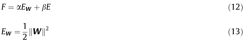
The relative size of  and
and  determines the proportion of the penalty term. If
  , the performance function is approximate to no regularization, meaning it minimizes the training error but maximizes the possibility of overfitting. If
  , it focuses on the limitation of the network, making the model’s prediction capacity poor. Therefore, knowing how to determine the values of and is necessary. In the framework of Bayesian analysis, MacKay deduces that [27]

where  , represents the valid weight and N is the total number of samples. H is the Hessian matrix of F:

The Hessian matrix is very computationally intensive, and Foresee F. Dan and Martin T. Hagan approximated the Hessian matrix with the G–N method, which greatly reduces the amount of computation [28]:

where J is the Jacobian matrix of the training error.
2.3.3. SCG algorithm
The SCG is an improved learning algorithm of standard BP. In the traditional gradient descent method, a direction of gradient descent is perpendicular to the previous direction, causing the global minimum difficult to approximate. The conjugate gradient method determined the new search direction by combining the new direction with the previous search direction. The conjugate gradient method is computationally intensive, requiring a new search in each iteration. The SCG proposed by Moller successfully avoids this drawback by adding a confidence interval to the conjugate gradient [29]. The adjustment method of the SCG algorithm is

where wk is a point in Wk, pk is the search direction, and θk is the search step size of iteration k.

where gk is the current gradient of the function, and Hk is the Hessian matrix of iteration k.
Set  . In order to ensure
  > 0, set =
  .
.
The step size θk can then be determined:

《2.4. Verification and comparison of different models》
2.4. Verification and comparison of different models
The predictive performance of each model was assessed by the correlation coefficient (R) (Eq. (21)), and the training performance of each model was compared by the mean square error (MSE) (Eq. (22)). The R and MSE were calculated in the Matlab R2016a program.

where  is the covariance of predicted effluent TN and actual effluent TN;
  and
and  are the standard deviation of predicted effluent TN and actual effluent TN, respectively; m is the number of the datasets; TNPn and TNAn are the predicted effluent TN and actual effluent TN for sample n.
《3. Results and discussion》
3. Results and discussion
《3.1. Feasibility of the FFNN model using actual operation parameters as main input variables》
3.1. Feasibility of the FFNN model using actual operation parameters as main input variables
The number of nodes in the hidden layer needs to be determined prior to application. With other parameters constant, the number of hidden layer nodes was selected as 3 to 12 for training, according to Eq. (2). Fig. 2 shows the MSE for the different number of hidden layer nodes after training. By comparison, the number of hidden layer nodes was selected as 8, and therefore, the base FFNN model’s structure was constructed with 6–8–1 (Fig. 1). Consequently, MSE obtained the lowest value.
《Fig. 2》

Fig. 2. MSE for FFNN with different hidden layer nodes.
《Fig. 3》

Fig. 3. Comparison of predicted results and actual values of FFNN.
To train and assess the base FFNN model, the data collected from the long-term laboratory simulation of the SBR were randomly divided into a training set (104 groups) and a testing set (20 groups). Fig. 3 indicates a consistent trend overall, and the predicted value on the left side (training set) was close to the actual value (R = 0.91973), indicating that it was feasible to build a simulation model by replacing DO with actual controllable operation parameters such as superficial gas velocity and anoxic time as the FFNN input.
The prediction curve of the testing set on the right was, however, far from the actual situation (R = 0.5057), indicating that the simulation model still had some problems such as overfitting or falling into local minimum value which could reduce the prediction performance. To solve these issues, three algorithms (L–M, BR, and SCG) were used to optimize the FFNN model. A more complicated data set was used to train the model, and more reasonable training mode for different algorithms was established to find the best algorithm for the model.
《3.2. Optimization of the FFNN model by L–M algorithm》
3.2. Optimization of the FFNN model by L–M algorithm
The data set were randomly divided into a training set (80%) and a validation set (20%). After optimization by trial method, the number of hidden layer nodes was set as 30, the minimum number of failure times was set as 100, and tansig was selected as the transfer function between the hidden layer and the output layer. After training (113 steps), the training stopped because the number of failure times exceeded the preset value, with a shared time of 1.0 s. The simulation results are shown in Fig. 4. The MSE was 0.000200, and the R value in the training set, the validation set, and the whole set were 0.93603, 0.92316, and 0.93392, respectively, illustrating a good performance in effluent TN prediction. Given the higher R value and faster convergence speed than previous model, the model optimized by the L–M algorithm not only avoided the local minimum effectively, but also improved the convergence speed to the global minimum.
《Fig. 4》

Fig. 4. FFNN simulating results based on L–M algorithm: (a) the training set (the output ≈ 0.88 × target + 0.075); (b) the validation set (the output ≈ 0.88 × target + 0.074); and (c) the whole set (the output ≈ 0.88 × target + 0.077). The line ‘‘Fit” refers to the relationship between the target and the output and the line ‘‘O = T” means the target is equal to the output.
《3.3. Optimization of the FFNN model by BR algorithm》
3.3. Optimization of the FFNN model by BR algorithm
The BR algorithm did not need a validation set, and therefore, the data were randomly divided into a training set (80%), and a testing set (20%). In the process of model debugging, it was found that when hidden layer nodes were less than 20, the R value was lower than 0.6, and the results indicated that the prediction ability was poor. With the number of hidden layer nodes increased to 30, the R value gradually improved. After the number of nodes exceeded 30, the R value increased insignificantly, whereas the training time extended significantly. Consequently, the number of hidden layer nodes was selected as 30. Tansig was selected as the transfer function, the upper limit of training steps was set to 1000, and the training time was 19 s. As shown in Fig. 5, the R value of the training set is 0.90232, whereas the R value of the testing set is 0.83000. It was determined that the performance of the model was better than that of the base model and worse than that of the model optimized by the L–M algorithm. The BR algorithm improved the model performance by restricting the complexity of the network, leading to a higher R value than the base model. Nonetheless, several relationships between input and output may be lost due to the regularization, particularly in the case whereby the complexity of the model’s structure was moderate.
《Fig. 5》

Fig. 5. FFNN simulating results based on BR algorithm: (a) the training set (the output ≈ 0.76 × target + 0.15); (b) the testing set (the output ≈ 0.75 × target + 0.15); and (c) the whole set (the output ≈ 0.76 × target + 0.15).
《3.4. Optimization of the FFNN model by SCG algorithm》
3.4. Optimization of the FFNN model by SCG algorithm
Similar to the L–M algorithm, the data set was divided into a training set (80%) and a validation set (20%). The number of hidden layer nodes was maintained at 30 to ensure the identical model structure with the three algorithms. Tansig was selected as the transfer function between the hidden layer and the output layer, and the minimum failure time was 100. The training stopped after 156 steps because the number of failure times exceeded the preset value, and the usage time was near to zero. As shown in Fig. 6, the R value based on the training set and the validation set were 0.91653 and 0.96276, respectively. The higher R value of validation set revealed an inexistence of the overfitting phenomenon. With these results, it was concluded that the prediction performance of the FFNN model was excellent.
《Fig. 6》
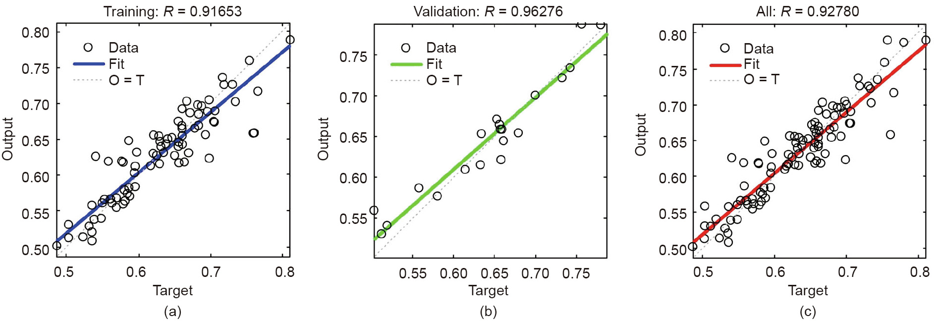
Fig. 6. FFNN training results based on SCG algorithm: (a) the training set (the output ≈ 0.84 × target + 0.1); (b) the validation set (the output ≈ 0.88 × target + 0.079); and (c) the whole set (the output ≈ 0.85 × target + 0.092).
《3.5. Comparison of three optimization algorithms》
3.5. Comparison of three optimization algorithms
The relevant training parameters of FFNN, based on different optimization algorithms, are summarized in Table 3. The results showed that in the training period, all three FFNN models with optimization algorithms had satisfactory MSE (< 0.001), and all gave better performances than the model without the algorithm optimization (MSE = 0.0037). Among them, the SCG algorithm was characterized by the shortest training time because of the rapid training method. The R values of FFNN, based on different optimization algorithms, are summarized in Table 4. In the training period, the three models obtained R values of 0.93603, 0.90232, and 0.91653, respectively, which was similar to the base FFNN model. The results revealed the intense relationship between input (influent water parameters and operation parameters) and output (effluent TN) from the training set. In the prediction period (testing and validation), all of the FFNN models obtained a higher R value than the base FFNN model. The results indicated that the prediction performance of the FFNN models for effluent TN was greatly improved by the optimization algorithms. The R value of the validation set of SCG was the highest in the three algorithms, and higher than the R value of the training set. The results demonstrated that the SCG algorithm obtained the most rapid calculation speed and outstanding prediction ability, and was an excellent algorithm for optimizing the FFNN model.
《Table 3》
Table 3 Relevant training parameters of FFNN based on different optimization algorithms.

《Table 4》
Table 4 R values in different datasets of FFNN based on different optimization algorithms.

《3.6. Comparisons with existing prediction models》
3.6. Comparisons with existing prediction models
Diverse simulation models have been proposed to achieve the prediction of effluent water quality in different wastewater treatment processes such as anaerobic–anoxic–oxic (A2 /O), SBR, and oxidation ditch with different model methods (traditional machine learning methods and ANN), and all the models were well suited to the specific environment. To predict NH4+ –N removal of slaughterhouse wastewater, a BP neural network model based on influent water quality and DO was proposed by Kundu et al. [30]. TN removal prediction of aerobic granulation was achieved using the ANN model based on influent water parameters [31]. A study by Ebrahimi et al. [32] proposed a multivariate regression model which could predict the effluent quality (biochemical oxygen demand (BOD), TP) of oxidation ditch. Nevertheless, the parameters selected in this study were mainly focused on DO and influent water parameters, but not controllability. The regulation strategies based on the models was lacking, because the feedback from the model was delayed.
Compared with previous studies, strong controllability and high prediction accuracy of simulation models were the two aspects highlighted in this study. This study is the first to demonstrate that TN removal performance could be controlled by the FFNN model based on actual controllable operation parameters such as superficial gas velocity and anoxic time, instead of DO, when considering the uncontrollability of DO. For the improvement of prediction accuracy, various algorithms were applied to optimize the FFNN model, and the model optimized by SCG was considered to have the highest prediction accuracy. To verify the advantage of the FFNN model optimized by SCG for effluent TN prediction, the FFNN model and other existing modeling methods, such as linear regression (LR), ridge regression, least absolute shrinkage and selection operator (Lasso) regression, support vector regression (SVR), and random forest (RF) were conducted (Table 5). The results showed that FFNN optimized by SCG was the best modeling method in this study, considering the lowest MSE and the highest R value of this model. It is reasonable that FFNN, optimized by SCG, could provide an accurate prediction of effluent TN, and fitted the real SBR process well.
《Table 5》
Table 5 Performance comparison of different prediction methods (R values are rounded to two decimal points).

In the future, the application of this prediction model could achieve the regulation of controllable operation parameters continuously, based on influent water parameters. Therefore, the effluent TN concentration could be maintained at a stable level and meet the relevant water quality standards. Furthermore, excessive aeration could be avoided effectively via continuous regulation of the operation parameters [33]. Finally, the energy consumption of controllable operation parameters would be minimized.
《4. Conclusions》
4. Conclusions
In this study, a SBR simulation model was developed, and the suitable control of effluent TN concentration and energy consumption were achieved after a long-term simulation of the SBR process. Superficial gas velocity and anoxic time were selected as the main input parameters of the FFNN model instead of DO, to improve the controllability of the model. Furthermore, SCG was selected as the algorithm for the optimization of the FFNN model because of the fastest calculation speed and outstanding prediction ability. Finally, the optimized FFNN model exhibited an excellent prediction capacity of effluent TN and optimal operation parameters. The findings of this study could provide a valuable solution for the stable operation and energy saving of WWTPs according to influent quality and effluent standards.
《Acknowledgements》
Acknowledgements
This work was funded by the Major Science and Technology Program for Water Pollution Control and Treatment (2017ZX07201003), the National Natural Science Foundation of China (51961125101), and the Science and Technology Project of Zhejiang Province (2018C03003).
《Compliance with ethics guidelines》
Compliance with ethics guidelines
Zihao Zhao, Zihao Wang, Jialuo Yuan, Jun Ma, Zheling He, Yilan Xu, Xiaojia Shen, and Liang Zhu declare that they have no conflict of interest or financial conflicts to disclose.
《Appendix A. Supplementary data》
Appendix A. Supplementary data
Supplementary data to this article can be found online at https://doi.org/10.1016/j.eng.2020.07.027.


 京公网安备 11010502051620号


