

《1. Introduction》
1. Introduction
The popularization of electric vehicles (EVs) is a worldwide strategy to reduce the dependence on fossil fuels and alleviate environmental pollution. Rechargeable lithium-ion batteries are considered as the most viable power sources for EVs [1–4]. With the wide adoption of EVs, we are beginning to see an increasing number of safety accidents caused by lithium-ion batteries in EVs around the world. These accidents tarnish the reputation of EV and battery manufacturers and harm public confidence in EV acceptance. Some accidents are caused by one type of electrical faults in batteries, that is, external short circuit (ESC). ESC faults can be triggered under any circumstances, for example, deformation of a battery pack during EV collision and water or oil leakage in a battery pack. Once an ESC fault occurs, it may cause a dramatic increase in battery temperature, which would lead to thermal runaway [5,6]. Therefore, it is necessary to study the thermal behavior of batteries under ESC faults for battery safety management.
《1.1. Literature review and motivations》
1.1. Literature review and motivations
Many researchers studied exothermic reaction mechanism and thermal responses as batteries generate tremendous heat under abusing conditions [7–9]. Ren et al. [10] developed a coupled electrochemical–thermal model to quantify heat generation rates of each heat source during the process from overcharge to thermalrunaway. Zhao et al. [11] studied the nail penetration test using a coupled three-dimensional (3D) multi-scale electrochemical– thermal model to illustrate the strong coupling relationship between thermal response and electrochemical behavior. Chen et al. [12] developed a multi-layer 3D thermal model to simulate temperature distribution in a battery at the occurrence of an internal short circuit. Zhu et al. [13] studied overcharge-induced thermal runaway by conducting overcharge experiments and found that side reactions dominate temperature rise before thermal runaway. In the abovementioned studies, complicated coupled electrochemical–thermal models were established to depict the thermal behaviors of batteries under abuse conditions. Generally, these models are computationally intensive and not suitable for real-world EV applications.
Many other researchers studied ESCs and mainly focused on ESC experimental methods, ESC behaviors and hazard analysis, and modeling and fault diagnosis [14–21]. Rheinfeld et al. [14,15] employed a quasi-isothermal ESC testing method to study the influence of material transport properties on transient shortcircuit behavior, and established a homogenized physical–chemical model to simulate the ESC process. In Refs. [16,17], ESC experiments were conducted to investigate electrical and thermal behavior under different ambient temperatures, initial states of charge (SOCs), and external resistances during the ESC process. Kupper et al. [18] proposed a physicochemical pseudo-3D multiscale model to describe thermodynamics and kinetics of main and side reactions in a battery cell under ESC conditions. In our previous research, we developed a fractional-order model to describe electrical characteristics of battery cells under ESC conditions, proposing a three-step diagnosis framework for an ESC fault [19] and later we proposed an online ESC detection method for a battery pack using an improved equivalent circuit model, which has high accuracy and generalization ability [20]. In Ref. [21], a neural-network-based method was proposed to estimate the ESC current of a battery cell using only voltage information.
In the above ESC studies, there is a lack of an effective thermal model to depict temperature rise in batteries under ESC conditions. A desirable model needs to be developed to achieve a balance between prediction accuracy and computational cost compared with complicated electrochemical–thermal models. In real-world EV applications, since not all battery cells are equipped with temperature sensors due to space limitation and manufacturing cost, temperatures of battery cells should be able to estimate only using current or voltage information. This motivates our development of a novel thermal model to predict temperatures with high accuracy and low computational burden to fill the gap in ESC studies.
《1.2. Original contributions》
1.2. Original contributions
The paper attempts to make the following three contributions: Firstly, ESC experiments of battery cells under different initial SOC values (20%, 40%, and 80%) and different ambient temperatures (–10, 10, 20, and 40 °C) were performed to establish an ESC database for building and validating the proposed thermal model. Secondly, an extreme learning machine (ELM)-based thermal (ELMT) model was explored to predict battery temperature under ESC conditions. Compared with the conventional ELM, the activation function was replaced with a lumped-state physical thermal model to better capture the battery temperature change. Finally, the proposed ELMT model was validated using the experimental data in terms of model fitting and prediction accuracy as well as computational cost. To demonstrate the effectiveness of the ELMT model, we compared the performances of the ELMT model with those of a multi-lumped-state thermal (MLT) model optimized by the genetic algorithm (GA).
《1.3. Organization of the paper》
1.3. Organization of the paper
In Section 2, the experimental results of batteries under ESC conditions are systematically presented and analyzed. Then, an ELMT model is proposed and explained in detail in Section 3. In Section 4, the proposed model is validated using data under different initial SOC values and ambient temperatures. Conclusions are summarized in Section 5.
《2. Experimental study》
2. Experimental study
To investigate the electrical and thermal characteristics of batteries under ESC conditions, we carried out ESC abusing tests under different experimental conditions. These conditions covered high, moderate, and low ambient temperatures (namely 40, 20, 10, and –10 °C, respectively), as well as high, moderate, and low SOCs (namely 80%, 40%, and 20%, respectively). Under each condition, we repeated the ESC test twice and their experimental results were denoted as group 1 and group 2. The data will be used to train and validate the proposed model in this paper. Table 1 describes the detailed specifications of the 18650 type Li(Ni0.5Co0.2Mn0.3)O2 battery cells studied in this paper.
《2.1. Experiment platform of ESC test》
2.1. Experiment platform of ESC test
As shown in Fig. 1, an ESC test bench has been established to study the characteristics of batteries under ESC conditions. In our previous work [20], we employed a similar platform to carry out the ESC test of battery packs, which has been illustrated in detail. In this paper, we focus on the ESC test of battery cells and briefly explain that the configuration of the experimental platform includes: ① an ESC test controller; ② a compressor supplying air source to the controller; ③ an explosion-proof thermal chamber; ④ current, voltage, and temperature sensors; and ⑤ a highprecision data acquisition system.
The data acquisition instrument was started to record experimental data once the contactor (shown in Fig. 1) was closed, where the contactor driven by the ESC test controller is used to make the connection of the positive and negative of battery cells, imitating ESC faults in EVs. Meanwhile, battery current, voltage, and temperature were measured by relevant sensors. When the current and voltage reduced to 0 A and 0 V indicating the battery was destroyed, the ESC testing was ended manually.
《Table 1》
Table 1 Specifications of the nickel–cobalt–manganese-based cathode materials battery.
《Fig. 1》

Fig. 1. Battery ESC test bench.
《2.2. Analysis of experimental results》
2.2. Analysis of experimental results
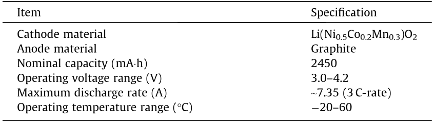
The current and temperature data are shown in Figs. 2 and 3, respectively. Figs. 2(a) and (b) show the results of group 1 under different SOCs at the ambient temperatures of 20 and 40 °C; Figs. 2(c) and (d) show the results of group 1 under different SOCs at the ambient temperatures of 10 and –10 °C. Similarly, Fig. 3 shows the results of group 2 under different SOCs and different ambient temperatures. As shown in Figs. 2 and 3, once the ESC occurred, the current increased rapidly within 1 s and the peak current can reach nearly 150 A (about 61 C-rate). The large current generated Joule heat accumulating inside batteries, causing the temperature of batteries to rise rapidly. After the current reached the peak, it was gradually decreased. As described in Ref. [18], the reason for current being reduced after the peak is that the high temperature can cause a ‘‘shut down” effect of battery separator, reducing the rate of lithium-ion diffusion and migration. Eventually, the current experienced a ‘‘discharge plateau” and then dropped to 0 A, indicating that the battery was damaged.
We can have the following observations from Figs. 2 and 3: ① Under the same SOC and ambient temperature conditions, the results of two groups exhibit good repeatability; ② under the same ambient temperature, battery cells with lower SOC discharge longer than those with higher SOC; ③ cells with higher SOC may have a larger rate of temperature rise under all ambient temperatures. More ESC test results were analyzed in detail in our previous work [19–21].
《Fig. 2》
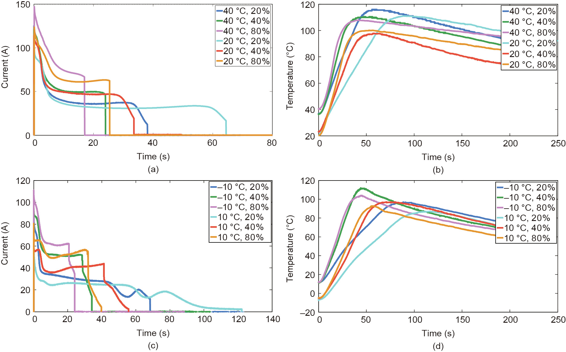
Fig. 2. Current and temperature of battery cells during ESC under different ambient temperatures and SOCs (group 1). (a) Current at 20 and 40 °C; (b) temperature at 20 and 40 °C; (c) current at –10 and 10 °C; (d) temperature at –10 and 10 °C.
《Fig. 3》
Fig. 3. Current and temperature of battery cells during ESC under different ambient temperatures and SOCs (group 2). (a) Current at 20 and 40 °C; (b) temperature at 20 and 40 °C; (c) current at –10 and 10 °C; (d) temperature at –10 and 10 °C.
《3. Modeling and prediction of battery thermal behaviors》
3. Modeling and prediction of battery thermal behaviors
《3.1. Lumped-state thermal (LT) model》
3.1. Lumped-state thermal (LT) model
An LT model is employed to describe the temperature behavior of a battery cell under ESC faults. It is assumed that the temperature within a battery cell is uniform. According to energy conservation, a gross heat generated by a battery can be expressed as the convection heat and the generated heat, which is modeled by

where h is the convection coefficient; Tamb is the ambient temperature; T is the temperature of the cell; Cp, V, A, ρ, and t represent the battery specific heat capacity, volume, surface area, density, and time, respectively; q is the heat generation [22,23], which can be computed as

where  is irreversible heat generation associated with ohmic and kinetic losses across the cell,
 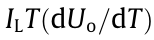 is the combined reversible heat generation associated with the electrochemical reaction, IL is the load current, Ri denotes the total impedance inside the battery, and Uo is the open-circuit voltage. In general, the irreversible heat generation includes two parts: ① Joule heat loss caused by the current flowing through the interface of the current collector and solid electrolyte interface (SEI) film; ② polarization heat loss caused by overpotential. The reversible heat generation is the electrochemical reaction heat generation caused by lithium-ions intercalation or deintercalation from positive and negative materials inside the battery.
In Eq. (2), researchers have proved that the reversible heat generation is much smaller than the irreversible heat generation under ESC conditions [16]. In this work, the ESC experimental data at 40% SOC and 20 °C in group 1 was used to calculate and compare the two parts of heat generation. Figs. 4(a) and (b) show the measured entropy coefficient  and results of reversible and irreversible heat generation, respectively.
It can be seen from Fig. 4(b) the irreversible heat generation  is much larger than the reversible heat generation
  . Therefore,
  in Eq. (2) is neglected. Then, substituting the reduced Eq. (2) into Eq. (1) and discretizing Eq. (1) in time, we have
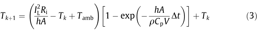
where Tk is the battery temperature at time instant k and  is the sampling period.
《Fig. 4》

Fig. 4. Results of heat generation. (a) Entropy coefficient; (b) reversible and irreversible heat generation.
《3.2. Description of ELM》
3.2. Description of ELM
Huang et al. [24] first proposed ELM to overcome the drawbacks of the single-hidden-layer feedforward neural network, for example, slow training speed, susceptibility to a local minimum, and sensitivity to the learning rate. The structure of a conventional ELM is shown in Fig. 5. In ELM, the weights connecting the input layer and the hidden layer and the bias of the hidden layer are randomly generated. Learning can be made more effectively without iteratively tuning, as the weights connecting the hidden layer and the output layer are identified by fitting the training data [25].
The input vector X and output vector Y of the ELM are defined as

where x and y are input and output data, respectively; n and m denote total data in the input and output layer, respectively.
《Fig. 5》
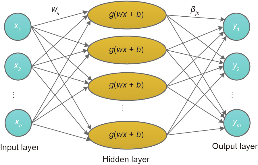
Fig. 5. Structure of conventional ELM. x and y are input and output data, respectively; n and m are total data in input and output layer, respectively; w is the weight connecting the input layer and the hidden layer; βjs is the weight connecting the hidden layer and the output layer; g(∙) denotes the activation function; b is the bias in the hidden layer; i denotes the input number; j denotes the sub-model number; and s denotes the data number in output layer.
The procedures for constructing an ELM are described as follows:
Step 1: Determine the number of neurons/nodes in the hidden layer, l.
Step 2: Randomly generate the weights w between the input layer and the hidden layer and the bias b in the hidden layer. The matrix w and vector b are shown as
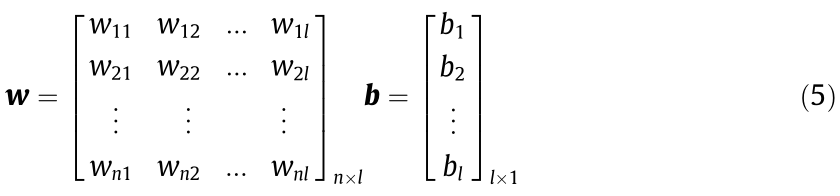
Step 3: Select a type of activation function g(∙) for computing the output.

where βjs is the weight connecting the hidden layer and the output layer, s is the data number in output lay (s = 1, 2, ..., m), i is the input data number, j is the sub-model number. If we define weight matrix β as

Eq. (6) can be expressed in matrix form as

where H = is the output matrix of the hidden layer.
Step 4: Determine the weights between the hidden layer and the output layer. The weight matrix β can be obtained by applying the least-squares fitting of Eq. (8) with the measurement data
matrix Y*.

The solution would be

where H + is the Moore–Penrose inverse of H.
《3.3. Proposed ELMT model》
3.3. Proposed ELMT model
In conventional ELM, the activation function is usually nonlinear and differentiable, including sigmoid function, hyperbolic tangent function, and Gaussian function [24]. Further research found that the activation function can be any nonlinear function or even discontinuous or non-differentiable function [25–28].
In this paper, we combined a physics-based LT model with the ELM, proposing an ELMT model to capture battery temperature under ESC conditions. Specifically, we replaced the conventional activation function of the ELM with the LT model previously introduced in Section 3.1. The ELMT model structure is shown in Fig. 6. In this model, we employed L sub-models, taking current Ik as the input and temperature Tk+1 as the output (k = 1, 2, ..., N – 1). N is the total number of temperature data. The L sub-models can be viewed as a type of activation functions of the ELM.
《Fig. 6》
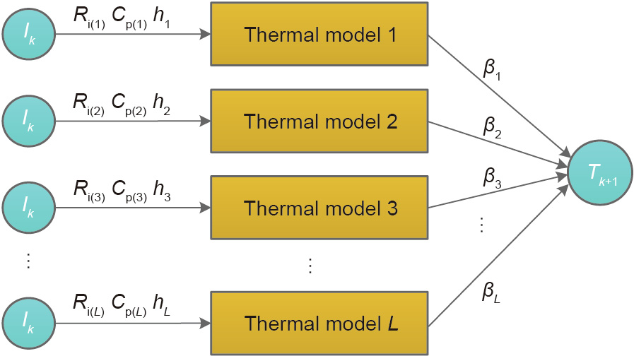
Fig. 6. Diagram of ELMT model. Ik : current at time instant k.
Based on Eq. (3) of the LT model and Eq. (6) of the ELM, battery temperature Tk+1 can be expressed as
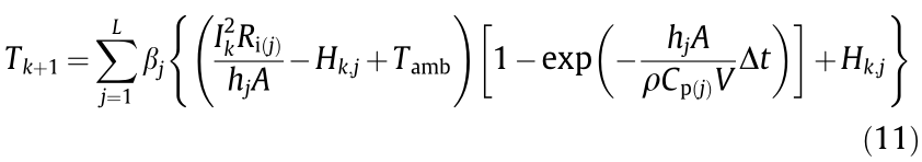
where j denotes the sub-model number (j = 1, 2, ..., L), Hk,j is the output of the jth sub-model in the hidden layer. The significance of the other parameters has been explained in Section 3.1. The recursive expression of Hk+1,j can be shown as

As a result, Eq. (11) can be rewritten as
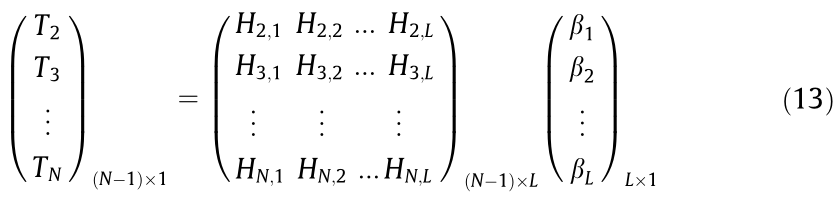
Eq. (13) shows that the temperatures at every time instant are regarded as the weighted sum of L sub-models. In this model, we can directly measure or calculate the battery mass, surface area A, and ambient temperature Tamb. The unknown parameter matrix P is shown as follows:
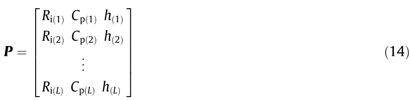
There are 3 × L parameters in the L sub-models that need to be determined. According to the principle of ELM, these parameters are assigned randomly within reasonable ranges and do not need to be tuned using the experimental data. This practice can significantly reduce the computational complexity of model parameterization. The ranges of these parameters are given based on prior knowledge [29,30]. For example, h is usually between 10 and 200W·m-2 ·K-1 under forced air convection. Therefore, the wide ranges of these parameters as shown in Table 2 are provided to cover a variety of battery operation conditions and obtain the optimal solution.
《Table 2》
Table 2 Parameter ranges of LT model.

The weights βj connecting the hidden layer and the output layer are determined by fitting the experimental data as in Eq. (10). In this paper, the number of LT model is set to 20 to balance the computational efficiency and model fidelity.
The advantages of the ELMT model are summarized as follows:
(1) Compared to general machine learning models, the ELMT model greatly improves the computation efficiency, as learning can be made more effectively without iteratively tuning parameters in Eq. (14).
(2) Since the ELMT model is a type of neural network model, it can achieve better accuracy by fitting the training data compared to the simple lumped thermal model.
(3) Compared to conventional ELM, the ELMT model employs the physics-based thermal model to replace the activation function, rendering its physical significance. The ranges of these weights w and bias b can be set based on the prior knowledge of the model parameters.
(4) The method to combine thermal model and conventional ELM can also be extended to other complicated electrical and electrochemical models, in which some parameters are difficult to determine. The proposed method can obtain an accurate model by setting parameters in reasonable ranges.
《3.4. MLT model》
3.4. MLT model
To demonstrate the advantages of the ELMT model, an MLT model is employed as the benchmark for comparison. The MLT model consists of five LT models and the MLT model structure is the same as that of the ELMT model shown in Fig. 6. However, in the MLT model, the parameters, for example, Ri, h, Cp, and βj, can be tuned to fit the experimental data. For a fair comparison, a total of 20 tunable parameters in the MLT model are the same as those of the ELMT model (20 weights βj connecting the hidden layer and the output layer).
The parameters of the MLT model are identified using GA, which is a commonly used nonlinear heuristic optimization algorithm [29]. In GA, the parameters are tuned to minimize a leastsquares objective function J defined as
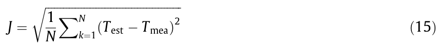
where Test is the estimated temperature and Tmea is the measured temperature.
Overall, there are 20 tunable parameters in both ELMT and MLT models. The major difference between the two models is the method to tune the parameters. For the ELMT model, the parameters are obtained through a one-shot least-square fitting without tuning iteratively; for the MLT model, the parameters are obtained through a process of iterative optimization.
《4. Evaluation of the proposed method》
4. Evaluation of the proposed method
In this section, we used the experimental data presented in Section 2 to evaluate the proposed ELMT model. We checked both the fitting accuracy of the model under the original training data in group 1 and the prediction accuracy under new data acquired from different battery cells in group 2. In all fitting and prediction cases, the MLT model is used as the benchmark to evaluate the ELMT model.
《4.1. Fitting accuracy》
4.1. Fitting accuracy
The experiment data in group 1 was used to examine the fitting accuracy of the ELMT model, which indicates the capability of the model to capture the fundamental dynamics of battery thermal behavior under ESC conditions. Fig. 7 shows the model fitting results of the ELMT and MLT models under the ambient temperatures of 20 and 40 °C and 80%, 40%, and 20% SOCs, and Fig. 8 presents the results under the ambient temperatures of –10 and 10 °C and the same SOCs as those in Fig. 7. Besides, the inset (i) of each subplot represents the errors of the ELMT model, and inset (ii) represents those of the MLT model. It can be seen that the temperature errors of the ELMT model were less than 4 °C, whereas those of the MLT model can be as high as 25 °C.
《Fig. 7》
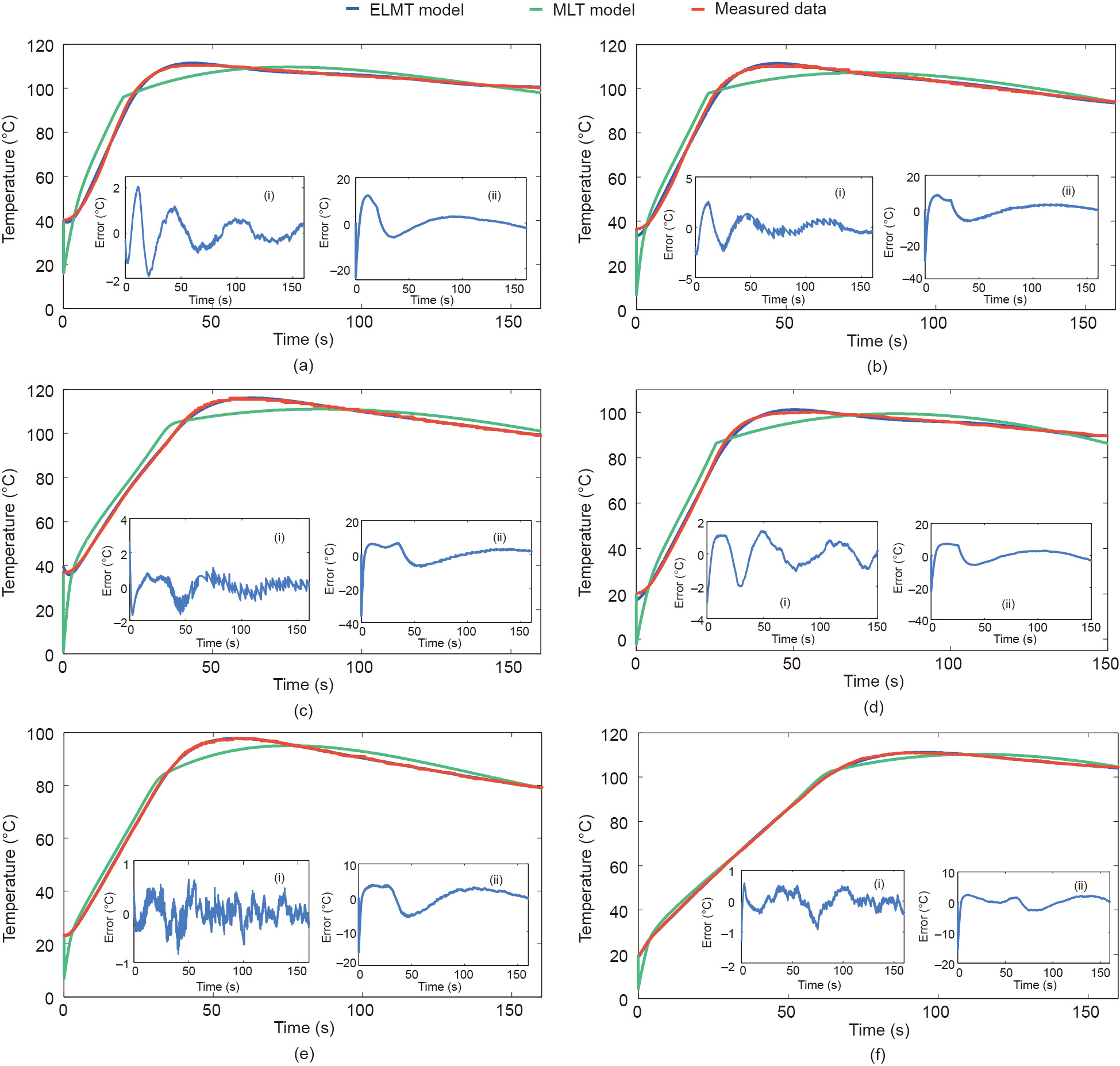
Fig. 7. Model fitting results with different SOCs under ambient temperatures of 20 and 40 °C. (a) 80% SOC at 40 °C; (b) 40% SOC at 40 °C; (c) 20% SOC at 40 °C; (d) 80% SOC at 20 °C; (e) 40% SOC at 20 °C; (f) 20% SOC at 20 °C.
《Fig. 8》
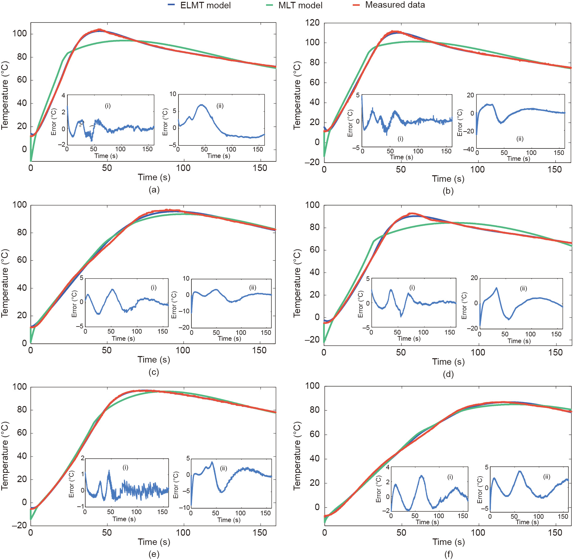
Fig. 8. Model fitting results with different SOCs under ambient temperatures of –10 and 10 °C. (a) 80% SOC at 10 °C; (b) 40% SOC at 10 °C; (c) 20% SOC at 10 °C; (d) 80% SOC at –10 °C; (e) 40% SOC at –10 °C; (f) 20% SOC at –10 °C.
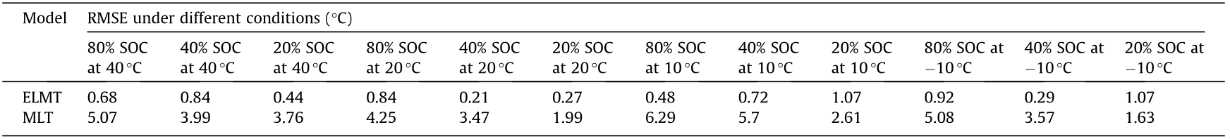
Table 3 compares the root mean squared error (RMSE) of the two models under different conditions. Table 4 shows the average RMSE results under each ambient temperature as well as all conditions. It can be seen that the ELMT model has better fitting accuracy than the MLT model under all the conditions, namely the average RMSE of the ELMT model is 0.65 °C whereas that of the MLT model is 3.95 °C (Table 4). Thus, the ELMT model has a better ability than the MLT model with the same number of tuning parameters to capture the temperature response under all battery initial SOCs and ambient temperatures.
《Table 3》
Table 3 Model fitting RMSE under different conditions.
《Table 4》
Table 4 Average RMSE results under different ambient temperatures.

In terms of the computational efficiency of model training/fitting, the training time of the two models under different conditions are shown in Table 5. The computing time is recorded from the start of the program to the end of the program based on MATLAB 2013b (MathWorks, USA). All results were obtained on the platform of a ThinkPad T470 (Intel®CoreTM i7-7700HQ central processing unit (CPU) 2.8 GHz, random access memory (RAM) 16 GB, solid state drive (SSD) 500 GB).
《Table 5》
Table 5 Comparison of computing time under different conditions.

It is clear that the ELMT model takes less time to compute than the MLT model. As mentioned previously, the reason for the better computational efficiency of the ELMT model is that the majority of its parameters are randomly assigned without the need for training and the remaining parameters are obtained through a one-shot least-square fitting without the need for iterative tuning. On the contrary, the parameters of the MLT model are identified by using the more complicated iterative GA.
《4.2. Prediction accuracy》
4.2. Prediction accuracy
The experiment data in group 2 was used to evaluate the prediction accuracy of the ELMT model for the thermal behavior of a different set of batteries under the same ESC conditions. The same group of the data was also employed to the MLT model as the benchmark for comparison.
Fig. 9 shows the temperature prediction results of the two models under 20 and 40 °C at three different SOCs; Fig. 10 shows the results under –10 and 10 °C at the same SOCs. In each subplot of Figs. 9 and 10, inset (i) denotes the temperature prediction errors from the ELMT model; inset (ii) denotes the temperature prediction errors from the MLT model.
《Fig. 9》

Fig. 9. Temperature prediction results with different SOCs under ambient temperatures of 20 and 40 °C. (a) 80% SOC at 40 °C; (b) 40% SOC at 40 °C; (c) 20% SOC at 40 °C; (d) 80% SOC at 20 °C; (e) 40% SOC at 20 °C; (f) 20% SOC at 20 °C.
《Fig. 10》

Fig. 10. Temperature prediction results with different SOCs under ambient temperatures of –10 and 10 °C. (a) 80% SOC at 10 °C; (b) 40% SOC at 10 °C; (c) 20% SOC at 10 °C; (d) 80% SOC at –10 °C; (e) 40% SOC at –10 °C; (f) 20% SOC at –10 °C.
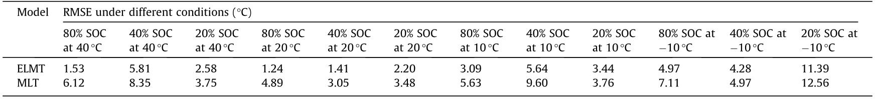
Table 6 shows the comparison of the RMSE results between the predicted values by the two models and measured data under different SOCs and ambient temperatures. Table 7 shows the comparison of the average RMSE results under each ambient temperature as well as all conditions. As shown in Table 7, the average RMSE of all conditions from the ELMT model is only 3.97 °C, whereas that from the MLT model is 6.11 °C. Thus, the ELMT model has better temperature prediction accuracy than the MLT model under all initial SOCs and ambient temperatures.
《Table 6》
Table 6 RMSE of predicted results of two models under different conditions.
《Table 7》
Table 7 Average RMSE results of two models under different ambient temperatures.

《5. Conclusions》
5. Conclusions
In this paper, we develop an ELMT model to capture the thermal behavior of lithium-ion batteries under different ESC conditions. In the proposed model, we replaced the conventional activation function with a physics-based LT model. Then, we systematically performed the ESC experiments of battery cells under different initial SOCs (20%, 40%, and 80%) and ambient temperatures (–10, 10, 20, and 40 °C). The experimental database is established to construct and evaluate the proposed model. To demonstrate the effectiveness of this model, we compared the ELMT model with an MLT model parameterized by GA. The two models are first evaluated by comparing their fitting training data (experimental data in group 1). The average RMSE of the ELMT model is 0.65 °C under all ESC conditions, whereas that of the MLT model is 3.95 °C. Besides, the computational complexity of the two models is also compared and it has been proved that the ELMT model has lower computing cost than the MLT model. Then, the two models are further evaluated for the prediction ability using the new data from different battery cells (experimental data in group 2). The average RMSE of the ELMT model is 3.97 °C under all ESC conditions, whereas that of the MLT model is 6.11 °C. All these results show that the ELMT model has better fitting and prediction accuracy as well as a lower computational burden than the MLT thermal model.
Our future work includes: ① studying on damage characteristics under different ESC stages; ② improving the generalization ability of the ELMT model to predict battery internal temperature.
《Acknowledgements》
Acknowledgements
Rui Xiong acknowledges support by the National Key Research and Development Program of China (2018YFB0104100). Ruixin Yang acknowledges support by the China Scholarship Council. The systematic experiments of batteries were performed at the Advanced Energy Storage and Application (AESA) Group, Beijing Institute of Technology.
《Compliance with ethics guidelines》
Compliance with ethics guidelines
Ruixin Yang, Rui Xiong, Weixiang Shen, and Xinfan Lin declare that they have no conflict of interest or financial conflicts to disclose.


 京公网安备 11010502051620号


