《1. Introduction》

1. Introduction

Underground construction has started attracting increasing attention with the gradual depletion of land space. However, the complex geological environment brings great challenges to urban underground transportation and tunnel construction projects. Various underground disasters, such as water inrush, mud surge, and roof collapse, can occur [1–5], causing huge risks to facilities and personnel [6–9].

Geophysical prospecting methods used in underground engineering are commonly classified into two categories: seismic and electromagnetic methods [10–19]. Seismic approaches, including advanced seismic prediction, scattering seismic computer tomography imaging, true reflection tomography, and land sonar [10– 15], mainly analyze the propagation characteristics of elastic waves in geological bodies, and infer their distribution, geometric morphology, and structural characteristics [10–18]. Electromagnetic approaches, such as the ground penetrating radar and the transient electromagnetic methods, generally deduce the characteristics of a geological body through difference in the dielectric constant and resistivity [14]. Both approaches can indirectly predict the existence of abnormal structures (e.g., water-rich areas) on a large scale.

With the emergence of new information technology like the Internet of Things, acoustic emission (AE) technology has been applied to the dynamic nondestructive testing of materials. It is mainly used in crack detection and fatigue fracture monitoring. AE technology can evaluate the integrity of components and the danger level of structures. Therefore, it has aroused great attention and gained rapid development in aviation, metallurgy, transportation, construction, and other fields. Based on the AE arrival time and other data, the source location and velocity structure can be iteratively solved. The inversion of the wave velocity field in the detected region defines abnormal (e.g., water-bearing) regions more intuitively, quickly, and accurately [20–26].

Jansen et al. [27] conducted ultrasonic imaging and AE monitoring for thermally induced microcracks in granite. Their study showed that both AE locations and slowness difference tomography clearly delineated the fracture plan. Nishizawa and Lei [28] employed the extended information criterion to advance the research on velocity tomography. Their meter-scale experiment revealed that this method provides an objective criterion for the selection of an optimum tomography solution. On a smaller scale, Lei and Xue [29] measured the ultrasonic velocity and attenuation during CO₂ injection into water-saturated porous sandstone using difference seismic tomography. They concluded that viscous losses due to fluid diffusion are of significant importance for compressional waves traveling at ultrasonic frequencies in porous rocks. Recently, Aben et al. [24] studied rupture energetics in crustal rock with laboratory-scale seismic tomography, in which a quasi-static rock fracture experiment combined with a novel seismic tomography method quantified the contribution of off-fault fracturing to the energy budget of a rupture.

In this paper, an improved three-dimensional (3D) AE tomography method based on the fast matching algorithm and least square quasi-Newton iteration is adopted to detect potential abnormal areas. This method is used for a joint inversion to obtain the 3D anisotropic P-wave structure using synthetic source locations and arrivals. By changing individual parameters, including the prior model, sensor configuration, inner event, origin model, ray coverage, and events location error, we explored the influence of different factors on imaging results.

《2. Methods》

2. Methods

In the synthetic experiment, through fast marching and standard optimization, the 3D anisotropic wave velocity imaging was conducted by combining active ultrasonic measurements with passive AE monitoring [30]. The inversion procedure is shown in Fig. 1. The improved algorithm contains the following five running steps: ① determining the initial environment and dividing mesh nodes; ② configuring the prior model; ③ collecting the required AE and ultrasonic data; ④ executing tomography calculations and establishing the velocity structure database; and ⑤ identifying abnormal regions from the tomography results. The inversion procedure is shown in Fig. 1.

《Fig. 1》

Fig. 1. Flowchart of the inversion algorithm. FaATSO: fast marching acoustic emission tomography using standard optimization.

(1) Determining the initial environment. First, we determine the size of the area to be tomographically measured. The size of the unit grid cube can be decided based on the condition of the structure and requirement for tomography precision. Generally, the denser the grid is, the higher the tomography precision will be; correspondingly, more computation is needed, and the processing requires more time. However, when mesh density is high enough, tomography precision does not be improved significantly with further mesh refinement. The matrix M of the same size as the grid node is established, and the index position in the matrix corresponds one-to-one to the grid node position. The grid nodes form a collection that is used as starting points in the search for the fastest waveform path between subsequent nodes. It is assumed that the propagation velocity of the P wave in the surrounding normal region is an unknown value, which is represented by V.

(2) Configuring the prior model. The prior model is configured based on the characteristics of the structure. Abnormal regions in complex structures are not known in practical applications. As a result, we have to infer the information of the unknown origin model by iterative calculation, and finally conclude the approximate model. In this simulation test, the complex structure was simulated as granite, and the abnormal area was the paste-filling area. In general, the P-wave velocities of granite and paste-filling are 4000 to 5500 and 1500 m∙s^–1 , respectively. Therefore, in the synthetic tests, the true model was set at 4500 and 1500 m∙s^–1 for granite (external region) and paste-filling (internal region), respectively. The average of the internal and external wave velocities was taken as the prior model.

(3) Collecting AE and ultrasonic data. Sensors, which are capable of actively transmitting and receiving the AE signal, were installed at different positions of the structure to be tested. In the 3D model, there are five source parameters (i.e., P-wave velocity V, AE source coordinate , and initial excitation time t₀). Therefore, the sensor number m must be an integer no less than 5. The sensor transmitting pulse signal is the active source whose coordinate and transmitting time are and , respectively. For the kth sensor S_k that receives the AE signal, the coordinate is , and the initial arrival time of the P-wave AE signal is . For an unknown source P₀ with position coordinates of , its initial excitation time is t₀.

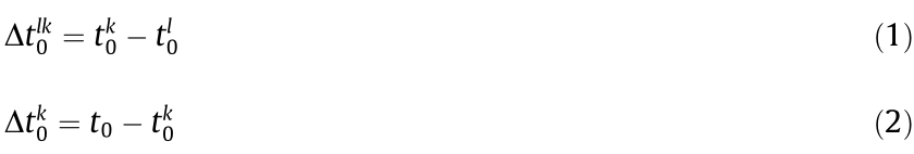
where  represents the difference of the actual arrival time between sensors  and S_k , while  is the actual arrival time difference between P₀ and S_k.

In this study, the coordinates of sensors and AE events (rough locations), as well as the arrival time differences of the sources, are all input data.

The P-wave velocity of each grid point in the structure was obtained by iterative calculation. These values were represented by different colors in the 3D diagram; the ray paths of the active sources and AE events to the receiving sensor were marked at the same time. Therefore, the boundary and location of the abnormal region in the complex structure can be intuitively separated via color difference. In addition, the properties of the abnormal region can be analyzed based on P-wave velocity values.

《3. Experiment》

3. Experiment

In an assumed 100 mm ×100 mm ×100 mm cube with a 60 mm (diameter) through-hole in the center, seven sensors were evenly arranged on each of the four vertical sides of the cube. In particular, when analyzing the influence of sensor arrangement on tomography results, another four sensors were uniformly distributed in the circular hole on the upper and lower surfaces of the cube. Sensors in synthetic tests have the active transmitted pulse function. Therefore, they can not only be used as the active AE source but also as receivers. Six hundred AE events were randomly generated inside the cube: 170 and 430 AE events inside and outside the internal hole area, respectively. The exact coordinate of each AE event was known and each event could be detected by every sensor.

The through-hole simulating the abnormal region in practical applications is hereinafter referred to as ‘‘internal,” and its P-wave velocity is represented by V_in; the structure outside the hole is referred to as ‘‘external,” and its P-wave velocity is represented by V_out. In synthetic tests, granite and paste-filling were considered to be the medium of the external and internal regions, respectively. To study the influence of different factors on tomography results, we quantitatively tested the prior model, sensor configuration, event distribution, origin model, ray coverage, and event location errors.

After calculating the tomography results of each synthetic experiment and obtaining the ray paths, we compared the inversion P-wave velocity V_t of each grid node with the actual value V_o of the origin model. If the difference between them is less than ±20%, the tomography result is regarded as valid. To quantitatively represent the effects of various influencing factors on inversion results, V_t of each grid in an experiment was compared with its corresponding V_o to calculate the tomography result accuracy under a specific condition.

《4. Results and discussion》

4. Results and discussion

《4.1. Prior model and sensor configuration》

4.1. Prior model and sensor configuration

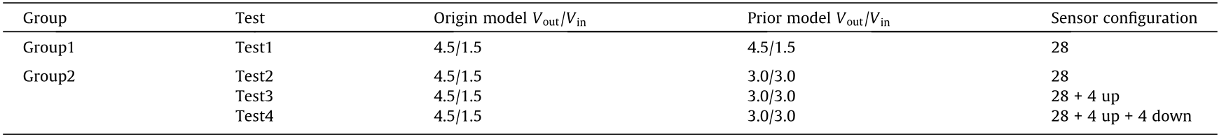
To evaluate the influence of the prior model and sensor arrangement on tomographic effects, two groups of four tests were conducted (Table 1). In addition to the 28 sensors placed around the cube, we placed four sensors above the through-hole area in Test3 and added another four sensors below the through-hole area in Test4. Test1 was compared with Test2 to analyze the influence of the prior model; Tests2, 3, and 4 were compared to investigate the effect of sensor configuration. In this scenario, the 170 AE events inside the through-hole area were eliminated, while the 430 events outside the through-hole area were retained. That is, there were no AE events inside the anomalous area.

《Table 1》

Table 1 Configurations of the model and sensor layout.

Before tomography inversions, we prepared the time arrivals of active ultrasonic measurements and AE events. The imaging results are shown in Fig. 2. Five tangent planes perpendicular to the z-axis represent the tomography results of the 3D P-wave velocity (Fig. 2). Propagation paths from the active pulse to the receiving sensor are shown as blue curves, and the ray paths of the AE event are presented by orange curves (one AE event was chosen randomly). Quantitative analysis of the P-wave velocity is shown in Fig. 3.

《Fig. 2》

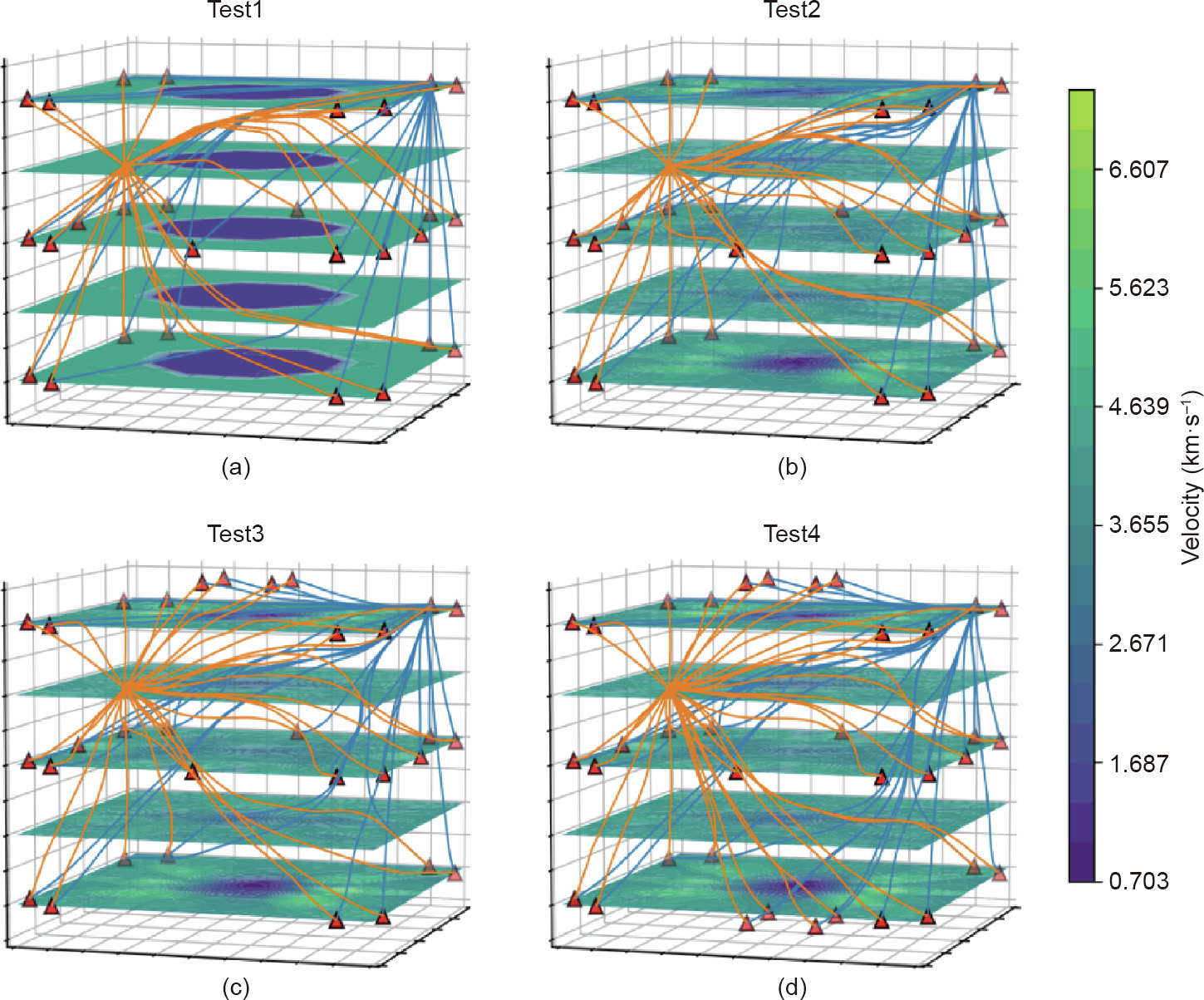
Fig. 2. Inversion results with different models and sensor layouts.

《Fig. 3》

Fig. 3. Quantitative influences of the model and sensor arrangement. (a) Correct rate for the V_in and V_out; (b) velocity distribution for the the V_in and V_out.

As shown in the tomographic results (Fig. 2), Fig. 2(a) presents a perfect mm circle; in Figs. 2(a)–(d), the circle disappeared. Moreover, when comparing the three tests in Group2, changing the sensor configuration did not work. Even when the sensor was placed on the paste-filling surface, the rays still bypassed the paste-filling area and passed through the rock. According to the tomographic results, relatively higher accuracies were obtained in the upper and lower sections of the structure. This is because the ultrasonic pulse signals of sensors arranged at the top and bottom of the hole bypassed the inside area and travelled through the outside in the upper and lower sections.

For Group1, when the prior model was equal to the origin model and the velocity precision was limited to 20%, the inverted V_out and V_in was 100% correct (Fig. 3). For the three tests in Group2, when the prior model was different from the origin model, the correct rate of V_in was less than 5% (Fig. 3), indicating that the abnormal velocity area cannot be accurately identified; however, the V_out still had relatively high accuracy.

《4.2. Events distribution》

4.2. Events distribution

Results in the previous section indicate that when the prior model is not close to the realistic case, the internal P-wave velocity values are calculated by iterative calculations based on input parameters. However, these results are not satisfying. The fact that the ray path of external events may not bypass the inside area could be one of the reasons affecting the tomographic effects. To examine whether this conjecture is true, i.e., whether there are differences in tomographic results in the presence and absence of internal events, the 170 inner events were added to the tests. We set another three tests corresponding to Tests2, 3, and 4 in Group2. Except for the 170 AE events located in the abnormal region (the through-hole area), all parameters remained unchanged (Table 2).

《Table 2》

Table 2 Parameters of influencing factors with inner events.

The test results are shown in Figs. 4 and 5. Different from sensors on the paste-filling surface, rays from inner events had to pass through the paste-filling area. However, the results were consistent with the previous ones, indicating that adding inner events did not improve the tomographic effects when the origin model V_out/V_in equaled 4.5/1.5.

《Fig. 4》

Fig. 4. Inversion results with different sensor layouts in the presence of inner events. (a) With 28 surrounding sensors; (b) with 28 surrounding sensors and 4 top sensors; (c) with 28 surrounding sensors, 4 top sensors, and 4 bottom sensors.

《Fig. 5》

Fig. 5. Quantitative influences of the sensor arrangement in the presence of inner events. (a) Correct rate for the V_in and V_out; (b) velocity distribution for the the V_in and V_out.

Tomographic effects obtained in the above experiments suggest that when the actual P-wave velocities in the external and internal (abnormal) regions were 4.5 and 1.5 km∙s^–1 , respectively, and the input V_out = V_in = 3 km∙s^–1 in the prior model, the inversion accuracy of the abnormal area was lower than 5%. Since the deviation of 20% is recognized as correct, changing the sensor layout or increasing the number of AE events in the abnormal region was almost ineffective.

《4.3. Origin model》

4.3. Origin model

We further analyzed the effects of the origin model and the prior model on tomography results. In the new tests, V_out/V_in in the origin model varies from 4.5/1.5 to 4.5/4.0. The prior model used the average of V_out and V_in. There were no AE events in the abnormal region. The experiment configurations are listed in Table 3.

《Table 3》

Table 3 Parameters of influencing factors with origin and prior models.

The tomographic results (Fig. 6) and the correct rate (Fig. 7) suggest that the inversion result was better when the difference between V_out and V_in was smaller (i.e., V_out/V_in was closer to 1). Especially, for Tests5 and 6, the accuracies of V_out and V_in reached almost 100%. Fig. 6 also shows that the ray paths of Tests5 and 6 are less curved or nearly straight.

《Fig. 6》

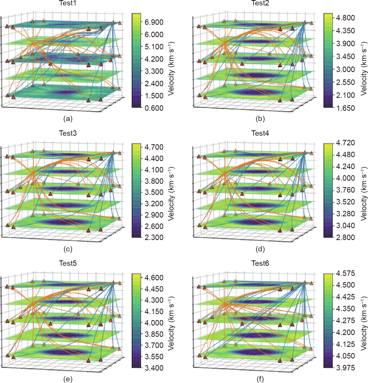
Fig. 6. Inversion results with different origin and prior models. (a) The origin velocity for V_out is 4.5 km∙s^–1 and V_in is 1.5 km∙s^–1 , the prior velocities for V_out and V_in are both 3.0 km∙s^–1 ; (b) the origin velocity for V_out is 4.5 km∙s^–1 and V_in is 2.0 km∙s^–1 , the prior velocities for V_out and V_in are both 3.25 km∙s^–1 ; (c) the origin velocity for V_out is 4.5 km∙s^–1 and V_in is 2.5 km∙s^–1 , the prior velocities for V_out and V_in are both 3.5 km∙s^–1 ; (d) the origin velocity for V_out is 4.5 km∙s^–1 and V_in is 3.0 km∙s^–1 , the prior velocities for V_out and V_in are both 3.75 km∙s^–1 ; (e) the origin velocity for V_out is 4.5 km∙s^–1 and V_in is 3.5 km∙s^–1 , the prior velocities for V_out and V_in are both 4.0 km∙s^–1 ; (f) the origin velocity for V_out is 4.5 km∙s^–1 and V_in is 4.0 km∙s^–1 , the prior velocities for V_out and V_in are both 4.25 km∙s^–1 .

《Fig. 7》

Fig. 7. Quantitative influences of the origin and prior models. (a) Correct rate for the V_in and V_out (values with 20% deviation are recognized as correct); (b) velocity distribution for the the V_in and V_out.

We narrowed the accepted velocity precision tolerance from 20% to 15% and finally to 1%. As shown in Fig. 8, the correct rates of V_out and V_in exceeded 50% in Tests5 and 6 when the precision tolerance was limited to 5% and 1%, respectively. When V_out/V_in was 4.5/4.0 or 4.5/3.5, namely (V_out –V_in)/V_out was less than 25%, the inversion results were very good despite there being only 28 sensors and the absence of inner events.

《Fig. 8》

Fig. 8. Quantitative influences of the origin and prior models for Tests5 and 6 with different precision tolerances.

As the difference between V_out and V_in gradually increased, the inversion accuracy of V_in decreased. However, as shown in the path diagram of Tests2, 3, and 4, the V_in (abnormal) area still could be distinguished (Fig. 6). The ray paths were tortuous and the internal area could not be detected when V_out and V_in were 4.5 and 1.5 km∙s^–1 , respectively.

Since the correct rate changes with the difference between V_out and V_in, we define the index E as

The inversion results corresponding to different E values from the above synthetic experiments are shown in Table 4.

《Table 4》

Table 4 E index and inversion effect corresponding to different origin models.

The tomography effects are intuitively presented by the increasing number of stars. The more stars the higher correct rate.

Among the four influencing factors—prior model, origin model, sensor configuration, and inner events—the origin model plays a decisive role in determining the tomographic results. When V_out/V_in in the origin model was 4.5/1.5, the tomographic results were not satisfying; the changes in the layout of sensors and the increase in inner events did not improve the tomography results. When the index E is higher than 50%, the results are not reliable; when E is between 25% and 50%, the results are reliable and stable; and when E is lower than 25%, the results are of relatively high accuracy. In addition, the accuracy of V_in in the upper and lower sections, as well as that of V_out, are relatively high, even though the tomography results are poor on the whole.

《4.4. Ray coverage》

4.4. Ray coverage

When the difference between the internal and external P-wave velocities was too large, the methods used failed to improve the results. The ray path of the P-wave changes in different media. A greater difference in the medium led to a more complex propagation mechanism and lower inversion accuracy, which is a common limitation of current AE wave velocity tomographic inversion methods [30].

Six additional tests (Table 5) were conducted in the synthetic structure. No AE events were generated inside the abnormal region, while AE events increased from 0 to 400 outside the abnormal region. The precision tolerance between the inverted P-wave velocity and the actual value was limited to ±5%. The results are shown in Figs. 9 and 10.

《Table 5》

Table 5 Parameters of influencing factors with ray coverage.

《Fig. 9》

Fig. 9. Inversion results with different ray coverage. (a) With only active ultrasonic measurements rays; (b) with ultrasonic measurements rays and 50 event rays; (c) with ultrasonic measurements rays and 100 event rays; (d) with ultrasonic measurements rays and 200 event rays; (e) with ultrasonic measurements rays and 300 event rays; (f) with ultrasonic measurements rays and 400 event rays.

《Fig. 10》

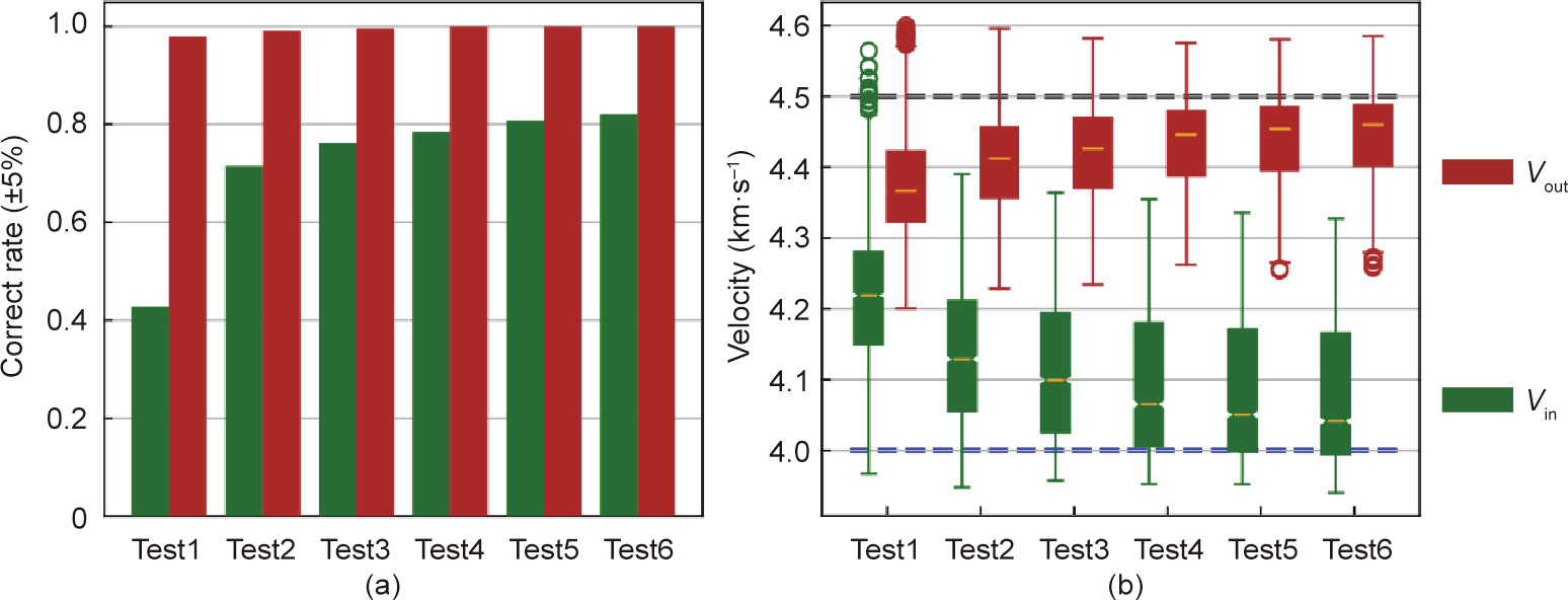
Fig. 10. Quantitative influences of the ray coverage. (a) Correct rate for the V_in and V_out (values with 5% deviation are recognized as correct); (b) velocity distribution for the the V_in and V_out.

The identification accuracy of the internal abnormal region increased with more outer AE events from Tests1 to 6 (Fig. 9). In addition, the V_in accuracy increased with AE events while the V_out accuracy remained relatively high (Fig. 10).

The above analysis indicates that when the origin model has a high inversion accuracy range, increasing ray coverage (by increasing the number of external AE events) can improve inversion accuracy. However, as the event number increases, the increasing rate of inversion accuracy tends to be flat (Fig. 10), meaning that it is difficult to significantly improve the correct rate by infinitely increasing the AE event number. As a result, a suitable number or range of AE events should be determined, so that a higher accuracy with a relatively small number of AE events can be obtained to save the cost in practical applications.

《4.5. Event location error》

4.5. Event location error

In synthetic tests, events were automatically generated, and their locations were therefore precisely known. However, the location of an AE event is unknown in practical applications. At present, there are multiple AE location methods [4,7–9]. Methods without pre-measured wave velocity greatly reduce the location error [7]. Nevertheless, there is still an error between the location results and the actual positions. Consequently, it is imperative to understand how the magnitude of the location error affects the inversion results.

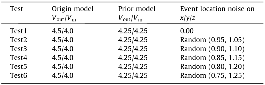
We investigated the effect of AE event location errors on tomographic inversion in two schemes, in which the number of external AE events was 400. In the first scheme (Scheme 1), all AE events had errors and the allowed location varying range expanded from (0.95, 1.05) to (0.75, 1.25), that is, the location error increase from ±5% to ±25% at the interval of 5%. In the second scheme (Scheme 2), the location error is fixed at ±20% and the number of mis-locating events increased from 50 to 300 at the interval of 50; the other conditions were the same as in Scheme 1. The configurations for Schemes 1 and 2 are listed in Tables 6 and 7, respectively. The results are shown in Figs. 11–14.

《Table 6 》

Table 6 Parameters of influencing factors with event location errors.

《Table 7》

Table 7 Parameters of influencing factors with mis-locating events.

《Fig. 11》

Fig. 11. Inversion results with different event location errors. (a) The event locations are without any error; (b) the event locations are scaled to 0.95–1.05 times of the true values; (c) the event locations are scaled to 0.90–1.10 times of the true values; (d) the event locations are scaled to 0.85–1.15 times of the true values; (e) the event locations are scaled to 0.80–1.20 times of the true values; (f) the event locations are scaled to 0.75–1.25 times of the true values.

《Fig. 12》

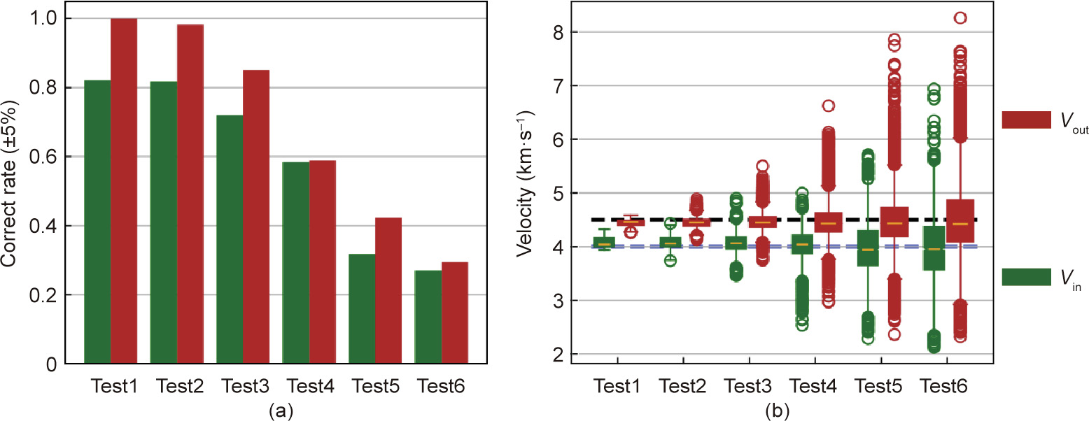
Fig. 12. Quantitative influences of the event location errors. (a) Correct rate for the V_in and V_out; (b) velocity distribution for the the V_in and V_out.

《Fig. 13》

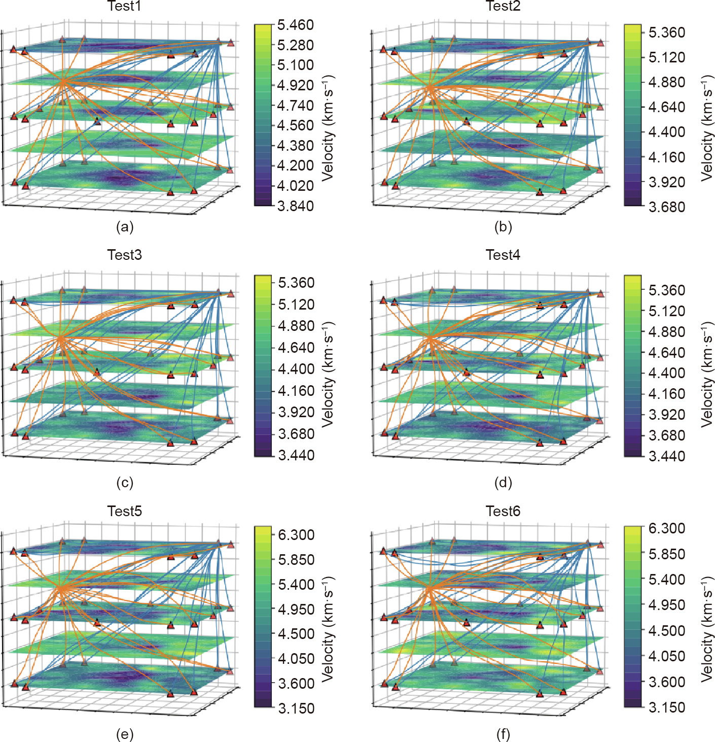
Fig. 13. Inversion results with a different number of mis-located events. (a) With 50 mis-locating events; (b) with 100 mis-locating events; (c) with 150 mis-locating events; (d) with 200 mis-locating events; (e) with 250 mis-locating events; (f) with 300 mis-locating events.

《Fig. 14》

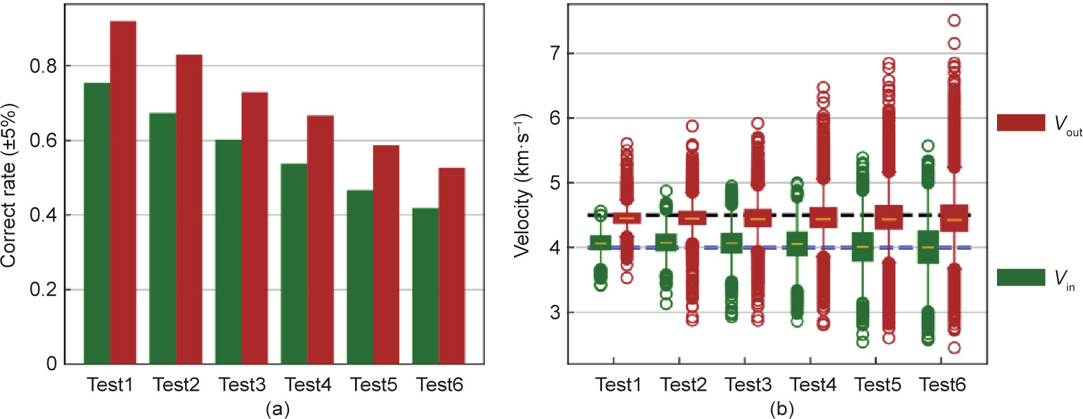
Fig. 14. Quantitative influences of the number of mis-located events. (a) Correct rate for the V_in and V_out; (b) velocity distribution for the the V_in and V_out.

The inversion results of Scheme 1 are shown in Fig. 11. From Tests1 to 6, the error range increased from ±5% to ±25%, and the tomographic effects became worse. For Test3, where the error range was ±10%, the cylindrical P-wave velocity of the abnormal region in the center could still be observed. When the error reached ±15% or more (i.e., in Tests4, 5, and 6), according to the inversion diagram, the internal and external P-wave velocity values increased, the boundaries of the internal and external wave velocity became blurred, and it was difficult to observe the abnormal region in the structure.

The quantified results of Scheme 1 (Fig. 12) show that the correct rate (5% deviation between the tomographic wave velocity and the actual value was recognized as correct) exceeded 70% when the location error was ±10%. In real applications, the location error in AE experiments can be easily limited to 10% [7]; for a sample of 100 mm, the location error can be less than 10 mm. Therefore, the AE P-wave velocity tomography method can reliably inverse the size and range of the abnormal region in a complex structure in the origin model with V_out/V_in of 4.5/4.0 and a reasonable location error.

The inversion results of Scheme 2 are shown in Fig. 13. As the number of error events increased from 50 to 300, the inversion effect became worse. The quantitative analysis chart (Fig. 14) reveals that the correct rate decreased from Test1 to Test6, which was slower than that in Scheme 1.

The comparison with Test6 in Section 4.3 (i.e., the number of external events was 430, and the event location was correct) suggests that erroneous location data have a great impact on inversion results. When the allowable error of the correct rate was 5%, the number of AE events changed from 430 correct to 350 correct and 50 errors, the accuracy rates of V_out and V_in dropped from 100% to 95% and from 83% to 75%, respectively. When the number of errors in AE events increased to 300 (with 400 total events), the accuracies of V_out and V_in reduced to approximately 30%; the inversion results were no longer reliable. Therefore, unreasonable, mis-located AE events affect the accuracy of tomographic inversion.

We noticed that in this synthetic experiment, V_out was always more correct than V_in. Due to the low wave velocity in the abnormal zone, rays bypass this area boundaries. Since very few rays pass through, there is a lack of ray data to calculate V_in, which ultimately results in less accurate results for V_in.

《5. Conclusions》

5. Conclusions

To analyze the influencing factors of AE wave velocity tomographic inversion, an improved 3D tomography method combining active and passive AE sources was adopted. A variety of comparative synthetic tests were performed, and quantitative analysis evaluated the influence of the following six factors: prior model, sensor configuration, inner events, origin model, ray coverage, and event location errors. The results show that optimal input parameters can significantly increase the tomography reliability of abnormal regions in complex structures.

Among the six influencing factors, the origin model plays a decisive role in the tomographic results. Therefore, if there is a big difference in P-wave velocity between the abnormal region and the surrounding region of the structure, it is be difficult to achieve desirable results. The difference between the internal and external wave velocities is represented by the index E. In general, when E ≥ 50%, the inversion result is not reliable. In a future study, we will consider adding weights to the low-speed region when the E value is too high, to reduce the E value and then to restore the inversion result corresponding to the correct wave velocity value.

When E is in a reasonable range, an origin model with a relatively high tomography accuracy is expected. When the number of external AE events reduces, the inversion accuracy decreases; the accuracy improvement rate becomes slower with an increasing number of events. Therefore, the appropriate number of events corresponding to a higher accuracy rate should be determined, to suggest an optimal scheme for practical applications. The inversion accuracy is also influenced if location errors increase. An acceptable range of location errors can allow a satisfactory accuracy. At the same time, by screening AE events in practical experiments, eliminating unreasonable AE events can improve tomographic inversion.

The premise of this velocity imaging method is that the material needs to be transversely isotropic with a vertical axis of symmetry (VTI), whose phase velocity is completely determined by the phase angle. In practice, the assumption of VTI geometry is particularly relevant to initially isotropic rock samples subjected to triaxial compression in the laboratory. In addition, this method is not very suitable for cases with major differences in wave velocity within a structure. It is more reliable and stable for cases with slowly changing wave velocity. In this study, we only tested a cylindrical anomalous area. The actual situation is much more complicated, and the tomography accuracy may be different in cases with anomalous shapes. Since the prior model is important for the inversion and we cannot accurately estimate the model in advance, a two-step strategy is suggested for rock experiments. That is, the ultrasonic survey should be performed first to estimate the approximate velocity in the structure, which is thereafter used as the prior model for later AE tomography.

《Acknowledgements》

Acknowledgements

The authors wish to acknowledge financial support from the National Natural Science Foundation of China (51822407, 51774327, and 51904334).

《Compliance with ethics guidelines》

Compliance with ethics guidelines

Longjun Dong, Xiaojie Tong, and Ju Ma declare that they have no conflict of interest or financial conflicts to disclose.