《1. Introduction》

1. Introduction

《1.1. Background and motivation》

1.1. Background and motivation

The electric power system (EPS) is a crucial part of the national energy supply, and policymakers are gradually realizing that heat supply also plays a key role in the energy system. The International Energy Agency reports that over half of global energy use is for heating [1]. A large proportion of the heat supply in high-density areas comes from district heating systems (DHSs), in comparison with the other heat alternatives—such as individual heat pumps, gas boilers, solar thermal heating, and electrical heating—that are often applied in low-density areas. Although different countries and areas use these heat supply methods in different proportions, the district heating approach has been proven to be extremely energy efficient [2].

Electricity and heat can be produced simultaneously with centralized energy generation and district heating infrastructures. In general, those two large energy systems—EPS and DHS—are tightly connected by combined heat and power (CHP, also known as cogeneration) plants and power-to-heat facilities. By 2050, CHP will provide 26% of electricity in the European Union. In Denmark, the government aims to achieve 100% renewable heat and electricity production by 2035 [3]. It is expected that EPSs and DHSs will impact each other to a greater extent in the energy production and consumption process in the near future. Therefore, the idea of the integrated heat and electricity system has attracted interest from practitioners and researchers.

Studies on different aspects of integrated heat and electricity systems are emerging, including modeling [4], state estimation [5], unit commitment [6], economic dispatch [7–9], market mechanisms [10,11], and planning [12,13]. Among them, modeling plays a fundamental and substantial role in the commercialization of integrated heat and electricity systems. Although EPS modeling has been studied thoroughly during the past decades, a great deal of research on DHS modeling is still ongoing. In general, DHS has three regulation modes, as shown in Table 1. Quality regulation employs a constant mass flow rate and variable temperature strategy [7]. Hence, the constraints in related optimization problems become linear and are thus easy to handle. However, a situation in which hydraulic conditions are predetermined may not lead to an economical solution. In contrast, quantity regulation maintains a constant supply temperature but regulates the quantity of mass flow rates. It has the advantages of flexibility and cost reduction because the mass flow rates will change according to the heat load, which will reduce the power consumption of the circulating water pumps. Apparently, greater economic efficiency and flexibility can be achieved by regulating both the temperature and the mass flow rates, which is referred to as quality–quantity regulation. So far, only a few works have explored the operation of integrated energy systems with a variable mass flow strategy [14–18]. Furthermore, efficient and scalable algorithms to solve the nonconvex and nonlinear network flow constraints are still under investigation. To this end, this paper proposes a convex model and an efficient algorithm for integrated heat and electricity systems under the quality– quantity regulation, in which the algorithm is expected to find the global optimum or a near-global-optimal feasible solution with a relatively small computational burden.

《Table 1》

Table 1 Different regulation modes in DHS.

《1.2. Literature review》

1.2. Literature review

The modeling of quality–quantity-regulated DHS is a type of pooling problem [19]. The pooling problem is a network flow problem that aims to find the minimum-cost way to mix several inputs in intermediate pools such that the output meets the demand or certain requirements. Mixing inputs involves mixing the product of the flow quantity and the feature. As a result, the pooling problem becomes a bilinear program. In DHS modeling, the nonconvex and nonlinear network flow hinders the problem from being solved efficiently. Among the nonconvex terms, the bilinear term, which comes from the product of the mass flow rate and the nodal temperature, is one of the most difficult to deal with.

Current achievements in dealing with the bilinearity of DHS optimization can be divided into four categories: nonlinear programming methods, generalized Benders decomposition, relaxation methods, and relaxation tightening methods. Nonlinear programming methods, such as the interior point method, sequential linear programming, and successive quadratic programming [14], are generally able to solve nonlinear programing with continuous variables, and are easy to implement with off-the-shelf solvers. However, they are only able to find local solutions and may have slow convergence or even convergence failure when the network becomes large.

Generalized Benders decomposition can solve certain types of nonlinear programming and mixed-integer nonlinear programming. To deal with the bilinearity from the product of the mass flow rate and the nodal temperature, Ref. [15] presents an iterative algorithm: By fixing one set of variables and solving the other set, and then vice versa, the two subproblems are iteratively solved until convergence is reached. However, the resulting solution cannot be ensured to be a global optimum or local optimum, and the convergence property requires further investigation.

In general, relaxation methods, such as conic relaxation [16,17] and polyhedral relaxation [18], enlarge the original nonconvex feasible set until it is convex. The relaxed problem becomes convex at the expense of sacrificing the feasibility of the solution to the original problem. The performance of relaxation methods largely depends on the relaxed boundaries, with tighter bounds leading to stronger relaxations. This gives rise to relaxation tightening methods, such as those shown in Refs. [18–20]. The core principle of such methods is to provide tighter bounds to enhance the relaxation. Among the relaxation tightening methods, branch and bound has been successfully implemented in the latest version of Gurobi—that is, Gurobi 9.0 [21]—to deal with bilinear programming. The bilinear solver in Gurobi 9.0 ensures a global optimum and can be used as a benchmark to evaluate the optimality of other methods. However, when dealing with large-scale problems, it may converge slowly.

《1.3. Contributions and the organization of this paper》

1.3. Contributions and the organization of this paper

In this paper, we first reformulate the classic quality–quantityregulated DHS optimization model through an equivalent transformation and the first-order Taylor expansion. Compared with the original model, which has two bilinear terms in each nonconvex constraint, the reformulated model has fewer bilinear equalities; more specifically, it reduces the bilinear terms by approximately half. The reformulation not only ensures optimality, but also may have advantages in reducing the computational complexities of the original problem. Next, we perform McCormick envelopes to convexify the bilinear constraints and obtain an objective lower bound of the reformulated model. To improve the quality of the McCormick relaxation, we employ a piecewise McCormick technique to reduce the McCormick volume by deriving stronger lower and upper bounds of the bilinear terms. The piecewise McCormick technique involves partitioning the domain of one of the variables in the bilinear term into several disjoint regions and determining the optimal region such that the bounds of the selected variable have been tightened. Thus, a strengthened lower-bound solution of the original problem is obtained. Since the strengthened lower bound may not be feasible, a heuristic bound contraction algorithm is further established to constrict the strengthened bounds of the piecewise McCormick technique and obtain a nearby feasible solution in an iterative way. Compared with nonlinear optimization [14] and generalized Benders decomposition [15], the proposed method is based on relaxation and piecewise techniques, which are more scalable, and thus avoids being trapped into local infeasibility. In contrast to current relaxation tightening methods, such as the one implemented in the Gurobi bilinear solver [21], the proposed tightening McCormick algorithm can achieve a comparable solution quality with better computational efficiency.

In summary, this paper makes three main contributions:

(1) A classic integrated heat and electricity operation problem with a quality–quantity-regulated DHS model is reformulated through a variable substitution and equivalent transformation, which largely reduces the bilinear complexity of the classic model.

(2) Based on the reformulated model, McCormick envelopes are applied to relax the remaining bilinear terms. To reduce the relaxation errors and strengthen the bounds used by the McCormick envelopes, a piecewise McCormick technique is proposed.

(3) To improve the feasibility of the solution, a bound contraction algorithm is designed to constrict the upper and lower bounds of the piecewise McCormick envelopes through a perturbation of the latest optimal results. Case studies show that the tightening McCormick method, which combines the piecewise McCormick technique with a bound contraction algorithm, quickly solves the problem with an acceptable feasibility check and optimality. Given its convex property, the tightening McCormick method is promising for large-scale integrated heat and electricity optimization and can allow economic analysis using shadow prices.

The remainder of this paper is organized as follows. Section 2 introduces the integrated operation problem with a DHS base model and a reformulated model. Section 3 details the convex relaxation and the tightening McCormick algorithm used to solve the integrated problem. Section 4 presents case studies, and Section 5 draws conclusions.

《2. Problem formulation》

2. Problem formulation

An integrated heat and electricity system consists of DHSs and local EPSs. A local EPS is part of the whole multi-area power system, which has one or more interfaces to exchange power with other parts of the whole power system. For DHS modeling, we present a base model first, which is a nonlinear optimization model without any relaxation of the constraints. Then, we derive an equivalent reformulated model of the DHS through the firstorder Taylor expansion and variable substitution. The reformulated model turns out to reduce the nonlinearity of the base model; that is, the bilinear terms in the base model are reduced by nearly half. For EPS formulation, we adopt a state-independent linear power flow model that considers the reactive power and voltage magnitude. The coupling elements connecting the two systems are CHP units. The operation problem determines optimal solutions with multiple objectives such as the minimization of fuel costs, power transaction costs with other interconnected power systems, and network losses. For notational simplicity, we build single-time horizon models for the DHS and EPS, respectively. Then, we extend the whole operation optimization to the multi-time horizon case and add the notation of time index t to all the decision variables.

《2.1. District heating system modeling》

2.1. District heating system modeling

In the quality–quantity-regulated radial district heating network, we regulate the mass flow rates through the circulating pump. Mass flow rate has a magnitude and direction. In this paper, we assume the magnitude of the mass flow rate to be variable, while the direction is fixed. This assumption is reasonable because frequent changes of direction will result in supply instability.

Base model:

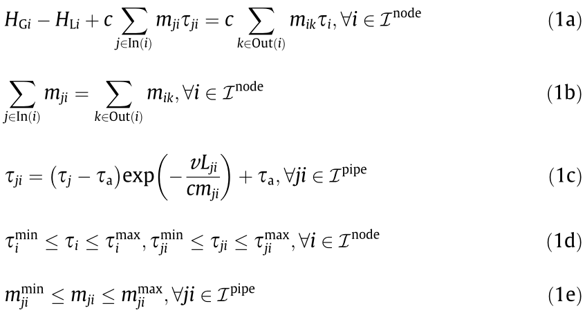
where H_Gi is the heat generation at node i, H_Li is the heat load at node i, c is the specific heat capacity of water, m_ji is the mass flow rate of water transferred from node j to node i in the pipeline of the heating network, is the outlet temperature of node i, is the outlet temperature of the pipeline from node j to node i, is the ambient temperature, v is the heat transfer coefficient per unit length, L_ji is the length of the pipeline from node j to node i, is the lower/upper limit of , and  is the lower/upper limit of m_ji . In(i)  is the set of indices of nodes flowing into node i in the heating network, and Out(i) is the set of indices of nodes flowing out of node i in the heating network.  e and  are the set of indices of nodes and pipelines in the heating network, respectively. Eq. (1a) defines the nodal heat balance, while Eq. (1b) defines the nodal flow balance. Eq. (1c) describes the process by which the water temperature drops along the pipeline, considering the heat-loss factors [22]. To be specific, the outlet temperature of the pipeline relies on the outlet temperature at the starting point of the pipeline, . If the pipeline length is longer, the heat transfer coefficient is larger, or the mass flow rate is smaller, the temperature drop (as well as the heat loss) will become more significant. Eq. (1d) are the minimum- and maximum-operating limits of the nodal outlet temperature and the pipeline outlet temperature. Eq. (1e) gives the minimum- and maximum-operating limits of the mass flow rates. Note that additional constraints that keep the supply nodal temperatures constant can be added into the base model; these would constitute the quantity-regulated model, whose computational complexity remains the same as the quality–quantity-regula ted model.

《2.2. DHS reformulation》

2.2. DHS reformulation

Nonconvexities of the DHS base model arise due to Eqs. (1a) and (1c). Eq. (1a) has the bilinear term , and Eq. (1c) has the exponential function exp(–vL/(cm)).

• To deal with the bilinear term, we introduce an auxiliary variable H=. With this variable substitution, it turns out that the bilinear terms are reduced.

• To deal with the exponential function term, we use the firstorder Taylor expansion to approximate the constraints in Eq. (1c).

By introducing auxiliary variables

In practice, the total heat transfer coefficient of pipeline v is very small. According to the Chinese design code for a city heating network [23], the heat transfer coefficient of the thermal insulation material should be less than 0.08 W·(m·K)^-1 . Thus, we assume that —an assumption that has been broadly studied and justified for heating networks [16,17,20]. Under this assumption, we can use the first-order Taylor expansion to approximate Eq. (5).

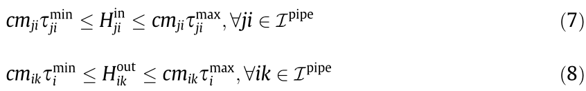
To transform the upper and lower limit constraints associated with temperature (i.e., Eq. (1d)) into constraints related to the heat power H, the following constraints are used:

Therefore, the district heating network formulation under quality–quantity regulation (the base model) can be reformulated as Eqs. (9a)–(9g), which represent the reformulated model.

Reformulated model:

It should be noted that Eq. (2) does not appear in the reformulated model. It has been eliminated because completely represents . Introducing and eliminating variables (Eq. (2)) will not influence the feasible region of the original problem. However, Eq. (9f) does not fall under the same case because is not only presented in Eq. (9f), but also appears in Eq. (9b). In the reformulated model (Eqs. (9a)–(9g)), the nonconvex quadratic constraints (Eq. (1a)) are converted into linear constraints (Eq. (9a)) and independent bilinear constraints (Eq. (9f)); thus, all constraints are linear except for Eq. (9f). It can be argued that the reformulated model is equivalent to the base model, with negligible errors from the first-order Taylor approximation.

《2.3. Electric power system modeling》

2.3. Electric power system modeling

A linear power flow [24] with accurate estimation of voltage magnitude is adopted to characterize the electric power network; this improves the direct current (DC) power flow results, since it accounts for the reactive power and voltage magnitude.

where is the active/reactive power generation at bus i,  is the active/reactive power load at bus i, is the active/reactive power flow across line ij, V_i and are the voltage magnitude and phase angle of bus i, respectively. g_ij is the conductance; b_ij is the susceptance. is the admittance of line ij, and  is the shunt admittance at bus i.   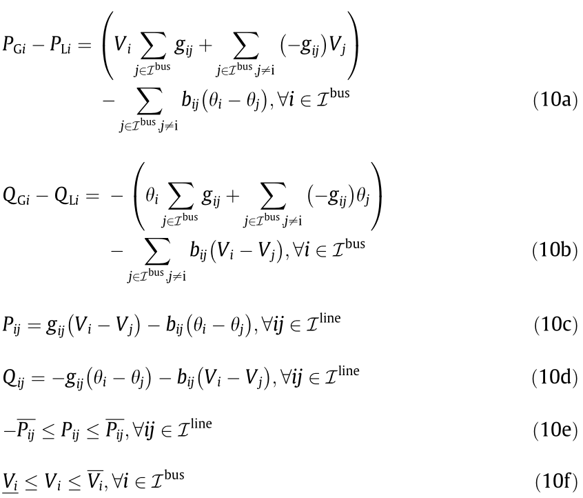is the lower/upper limit of V_i ,  is the upper bound of P_ij , and  and  are the set of indices of the buses and lines in the power network, respectively. Eqs. (10a) and (10b) define the nodal active and reactive power balance equations, respectively. Eqs. (10c) and (10d) present the branch active and reactive power, respectively. Eqs. (10e) and (10f) impose the active power limits of the transmission lines and the bus voltage magnitudes, respectively.

《2.4. Energy sources modeling》

2.4. Energy sources modeling

There are three typical types of energy sources in the integrated system: heating boilers (HBs), CHP units, and non-CHP thermal units (TUs). The variable cost of an HB is typically expressed as a linear function with respect to the heat output, whereas the variable cost may include fuel prices and taxes [25]. The generation cost of a CHP unit is usually formulated as a convex quadratic cost function of the power and heat output, including the product of the power and heat output [26]. The cost of each non-CHP thermal unit is modeled as either a quadratic or piecewise linear function in MATPOWER [27], and the quadratic form has been selected in this paper. The objectives of the above energy sources are described as follows:

where  are the cost functions of HB i, CHP i, and TU i, respectively.   and  are the generation cost coefficients of HB i, CHP i, and TU i, respectively.  is the heat output of heating boiler i,  is the active/reactive power output of CHP i,  is the heat output of CHP i, is the active/reactive power output of TU i, and  is the set of indices of TU.

The following constraints impose operational bounds for those energy sources, respectively. For CHP units, the bounds usually refer to the boundaries of the feasible region, whose shape may be either a line or a polygon [9], representing the relations between the heat output and the electricity output as well as their upper/ lower limits.

where  is the lower/upper limit of , and  and  are the parameters of boundary b of the feasible region at CHP unit i.  is the set of indices of boundary pairs in CHP unit i, and  is the lower/upper limit of .

《2.5. The operation problem》

2.5. The operation problem

The optimal operation problem in the integrated heat and electricity system is to minimize the fuel costs, the power exchange costs with other interconnected power systems, the network losses, and some other appropriate objective functions. The constraints include Eqs. (1a)–(1e) for the base model or Eqs. (9a)– (9g) for the reformulated model, in addition to Eq. (10), Eq. (12), and three other constraints regarding the nodal electricity/heat production equalities:

where  is the operation period,  is the set of indices of interfaces for power exchange, is the power bought from the outer grid at interface j,  is the power sold to the outer grid at interface j, and x represents decision variables. In the base model,  in the reformulated model,  are weight coefficients to adjust the weights of different objectives, which are set according to the operator’s preference.  refers to the power exchange cost at interface j, which is the difference between the costs of purchasing power from the grid and the revenues from selling power to the grid:

where is the price of buying/selling power from/to the outer grid at interface j at time t, and and  represent the total network losses at time t in the EPS and DHS, respectively. is defined as follows:

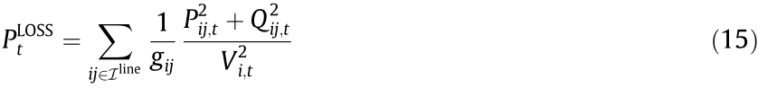
The literature contains several loss formulations and their variants; interested readers can refer to Ref. [28] for a thorough review. In this paper, we will adopt a common variant for Eq. (15), which assumes that all voltage amplitudes are equal to 1 per unit (p.u.) [29,30]. In general, voltage amplitudes are around 0.9–1.1 p.u., so the assumption is acceptable. It should be noted that so long as the loss formulation is convex, it can be applied to this problem.  is calculated as the difference between the total production and demand:

The problem (Eqs. (13a)–(13e)), whether with the DHS base model (Eqs. (1a)–(1e)) or the reformulated model (Eqs. (9a)– (9g)), is a nonconvex program with quadratic constraints. It is non-deterministic polynomial hard.

《3. Convex relaxation and the solution algorithm》

3. Convex relaxation and the solution algorithm

In the DHS reformulated model, the bilinear term is the only difficulty. An intuitive idea is to remove it—that is, remove Eq. (9f)— directly in order to check whether the bilinear constraints have a great impact on the quality of the solution. However, simulations show that removing bilinear terms leads to solutions with large violation errors to the constraints Eq. (9f). A classic way to relax the bilinear terms is to use McCormick envelopes. To improve the relaxation and reduce the McCormick volume, a piecewise McCormick technique is presented, since the sum of the smaller volumes is smaller than the big volume in the standard McCormick approach. The optimal results from the piecewise McCormick technique can be regarded as the relaxed global optimum, but may not be feasible for the reformulated model. Hence, a bound contraction algorithm is further proposed in order to strengthen the boundaries of the McCormick envelopes and find a feasible result near the relaxed global optimum.

《3.1. McCormick convex relaxation》

3.1. McCormick convex relaxation

We replace Eq. (9f) with the McCormick relaxation [31].

McCormick Model:

Under the McCormick relaxation, the reformulated model becomes a convex optimization problem, where the Karush–Kuh n–Tucker conditions are sufficient and necessary (under e.g., Slater’s conditions). Therefore, a global minimum can be achieved in the relaxed McCormick model. This global minimum can be regarded as a lower bound to the reformulated model. However, the McCormick relaxation still induces relatively large errors in the bilinear constraints.

《3.2. The tightening McCormick algorithm》

3.2. The tightening McCormick algorithm

We have obtained a solution through the convex McCormick model. Since the relaxed feasible region is not tight in the McCormick model, the solution may not be feasible due to violation of the bilinear constraints. To improve the quality of the relaxation, tighter lower and upper bounds are expected to help construct the McCormick envelopes. As such, we employ a piecewise McCormick technique and a bound contraction algorithm to improve the McCormick method.

3.2.1. The piecewise McCormick technique

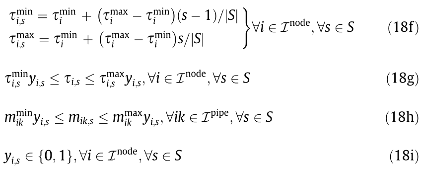
In the piecewise McCormick technique, the domain of one of the variables in the bilinear term is partitioned into several disjoint regions and the optimal region is determined such that the bounds of the selected variable have been tightened. A typical partition pattern is the uniform partition [32], where the problem size increases linearly with the number of partitions. Other partition schemes with adaptive segment lengths or partition-dependent bounds can also be applied to improve the performance [20].

The selected variables to be partitioned will influence the quality of the relaxation. In the district heating network flow optimization problem, the variable choice could be mass flow rates, nodal temperatures, or a combination of both. Finding an optimal set of variables for the best relaxation is beyond the scope of this paper. We will choose the nodal temperatures to partition. Let  and  represent the lower and upper bounds of variable  in partition s. A binary variable is assigned to each disjunction s. = 1 if the value of does belong to this disjunction; otherwise, = 0. The other variable of the bilinear term, m_ik, is also disaggregated as , where S is the set of indices of s.

Piecewise McCormick:

In the above formulation, if the binary variable is equal to 1, then all the variables in the sth partition—that is, —play dominant roles in deciding the values of . In comparison, the variables in all the other partitions are enforced to zero. Similarly, if = 1, then all the constraints in the sth partition are enforced, while the constraints in all the other partitions are neglected. The increasing number of binaries will lead to stronger relaxations, but at the cost of increased computational effort to solve the resulting mixed-integer problem. In general, the algorithm performs well with three partitions [32].

3.2.2. The bound contraction algorithm

The piecewise McCormick technique presents tighter upper bounds and lower bounds of the nodal temperatures, resulting in a stronger lower-bound solution of the reformulated model. To further reduce errors of the bilinear constraints, a feasible solution near the lower-bound solution is expected. Hence, we propose a bound contraction algorithm to iteratively strengthen the variable bounds and approach near-optimal results that violate the bilinear constraints less. The main idea of the bound contraction algorithm is that at each iteration n, the upper and lower bounds of the decision variables—that is, the mass flow rates and nodal temperatures—are updated according to the results from the last iteration n – 1 and a sequence of hyperparameters , where 0 < < 1. The principle in choosing the sequence is to gradually reduce the value of by in order to tighten the bounds [33]. To ensure the feasibility of the original problem, the updated bounds should be the intersection of the result-orientated bounds and the original bounds. Once the average relative error of the bilinear constraints (Eq. (9f)) is reached to an acceptable level , the algorithm can be terminated.

The abovementioned procedure is to search for a tighter lower bound. However, there is a need to obtain a feasible solution that can be regarded as an upper bound in order to assess the optimality gap , and that can act as another algorithm termination. The feasible solution can be recovered by fixing either the mass flow rates or the nodal temperatures obtained from the McCormick solution and re-optimizing the operation problem with the fixed value.

^a UB: upper bound; LB: lower bound.

《3.3. Overview of the proposed method and algorithm》

3.3. Overview of the proposed method and algorithm

Fig. 1 presents an intuitive illustration of the tightening McCormick algorithm, including the piecewise McCormick technique and the bound contraction algorithm. Fig. 2 illustrates the main procedure of the proposed method and algorithm. After model reformulation and convex relaxation, a convex McCormick model is formulated and provides an objective lower bound. To tighten the McCormick relaxation, stronger upper and lower bounds of the nodal temperatures are derived by partitioning the variable domain and are solved by means of the piecewise McCormick technique. Meanwhile, a feasible solution is expected to provide an upper bound and to form the stopping criterion together with the lower bound. The feasible solution can be recovered by fixing the mass flow rates and solving the resulting convex reformulation model, Eqs. (13a)–(13e), with Eqs. (9a)–(9g). The upper and lower bounds of the mass flow rates and the temperatures are successively tightened based on the bound contraction algorithm. Finally, the algorithm converges to a local optimum near the objective lower bound.

《Fig. 1》

Fig. 1. Illustration of the tightening McCormick algorithm. (a) The piecewise McCormick technique; (b) the bound contraction algorithm.

《Fig. 2》

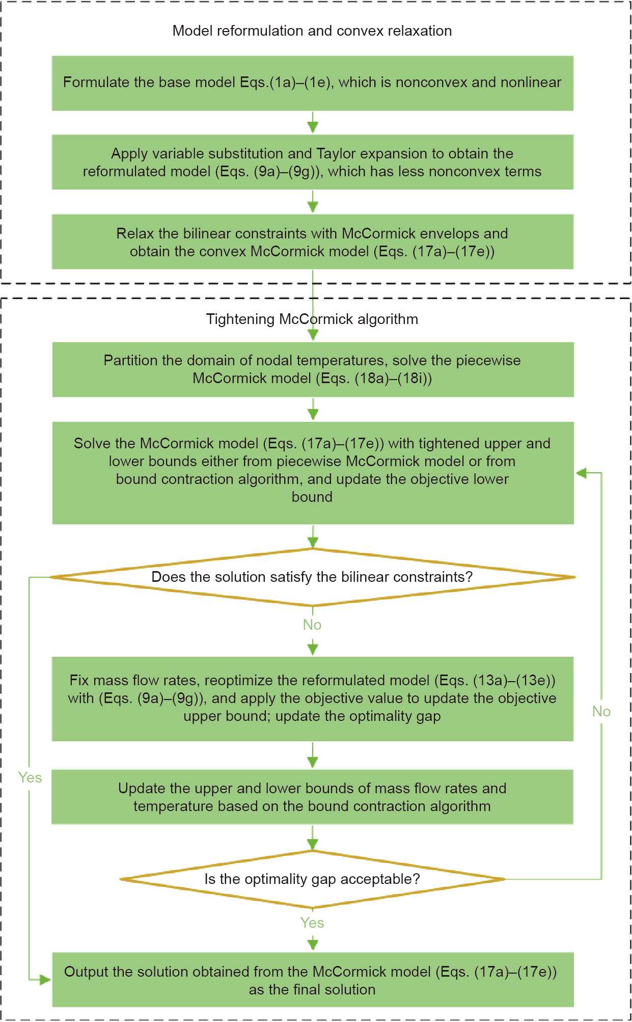
Fig. 2. The implementation flowchart for the proposed method and algorithm.

《4. Case studies》

4. Case studies

In this section, we compare the performance of several models, as shown in Table 2.

《Table 2 》

Table 2 Model settings for comparison.

We test these models in two integrated heat and electricity systems. One is a small-scale system with a 6-bus EPS and an 8-node DHS, as shown in Fig. 3. The 6-bus EPS is connected to the outer grid at bus 1. The 8-node DHS is modified based on a real DHS in Jilin Province, China [7]. There are two TUs, three electric loads, a CHP unit that connects the EPS and DHS, an HB, and three heat loads. The total heat load and electric load are shown in Fig. 4. The parameters are set to = 0.02, = 0.01, and = 0.0001. The other is a large-scale system consisting of a modified 118- bus EPS and a 33-node DHS in Barry Island [4]. The 118-bus EPS exchanges power with an outer grid at bus 69. The 33-node DHS disconnects branch number 25–28 to form a radial network. There are two CHP units and an HB in the DHS. Detailed data for the two integrated heat and electricity systems can be found in Ref. [34].

《Fig. 3》

Fig. 3. An integrated heat and electricity system with a 6-bus (i1–i6) EPS and an 8- node (n1–n8) DHS. Pd1–Pd3 refer to the electric demand 1–3; Hd1–Hd3 refer to the heating demand 1–3.

《Fig. 4》

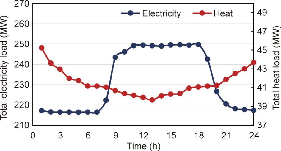
Fig. 4. The daily total heat and electricity profile.

《4.1. Optimality》

4.1. Optimality

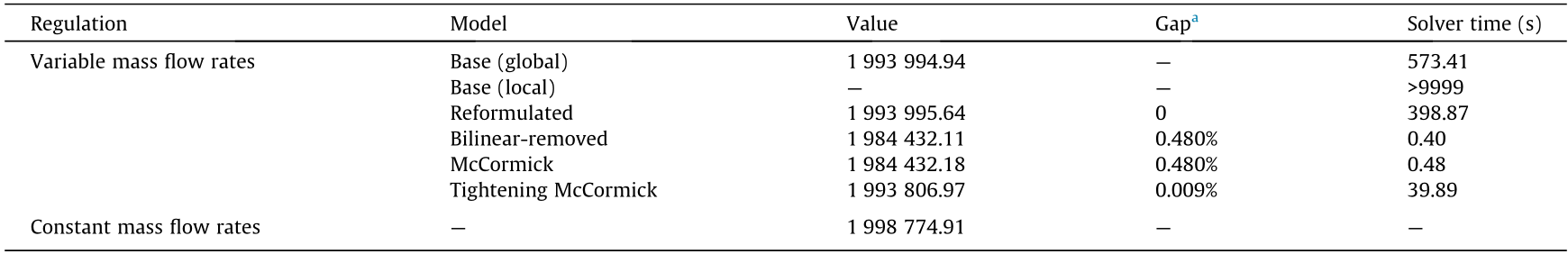
Table 3 and Table 4 show the optimal dispatch comparison in two cases, respectively. The base and reformulated models solved by the bilinear solver in Gurobi 9.0 provide the global optimal results. It is notable that there is almost no gap between those two models, which demonstrates that the reformulation preserves the same solution structure. As expected, the bilinearremoved model gives the lowest bound of the optimal solution, while the McCormick model provides a tighter lower bound. The base model solved by the local solver IPOPT presents an upper bound of the optimal solution. The tightening McCormick model has a small value gap and a fast solution time. When the network becomes large, the base model with the bilinear solver in Gurobi is time-consuming to solve. Since the problem is highly nonconvex, IPOPT even fails to converge in the large-scale case. However, with the convexified model, the tightening McCormick algorithm can be applied to the large-scale integrated system optimization with relatively small errors and is efficiently solved by off-the-shelf solvers. It is worth noting that, except for the preprocessed bound-strengthening process conducted by the piecewise McCormick technique, the remaining procedure in the tightening McCormick algorithm is actually applied on a convex model. In all, the tightening McCormick model performs well in terms of both solution accuracy and computational efficiency. Moreover, compared with using a global search, like branch and bound in Gurobi 9.0, the tightening McCormick model is a convex model, and it is easy to derive shadow prices for further economic analysis.

From the perspective of the regulation methods, it can be observed that the regulation with variable mass flow rates has lower costs than that with constant mass flow rates, as shown in Table 3 and Table 4, since the variable mass flow rate case results in more flexibility in both the mass flow rates and the nodal temperatures. A detailed day-ahead operation is demonstrated in Fig. 5, including the power output of each production unit, power selling to the grid, and the mass flow rates of typical pipelines.

《Table 3》

Table 3 Optimal dispatch comparison in the small-scale case.

^a Gap is defined as the relative difference value with respect to the value from the base (global) model.

《Table 4》

Table 4 Optimal dispatch comparison in the large-scale case.

^a Gap is defined as the relative difference value with respect to the value from the base (global) model.

《Fig. 5》

Fig. 5. The day-ahead operation of the small-scale case with different regulation methods. (a) Variable mass flow rates; (b) constant mass flow rates.

《4.2. Feasibility》

4.2. Feasibility

Fig. 6 shows violations of the constraints (Eq. (9f)) in two cases. Violations are represented by the errors of the bilinear constraints; that is, . Although Table 3 and Table 4 show that the bilinear-removed and McCormick models provide lower costs, it can be observed that their violations, as presented in Fig. 6, are huge. This is unacceptable when applied to real-world operations. However, the tightening McCormick model gives relatively small violation errors. The maximum errors are no more than 0.358%, and the average errors are less than 0.133% in both cases. Detailed error data is provided in Table 5 and Table 6.

《Fig. 6》

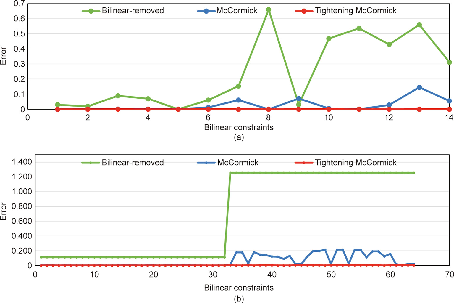
Fig. 6. Violations of constraints (Eq. (9f)) at hour 1. (a) The small-scale case; (b) the large-scale case.

《Table 5》

Table 5 Errors of the bilinear constraints (Eq. (9f)) during 24 h in the small-scale case.

《Table 6》

Table 6 Errors of the bilinear constraints (Eq. (9f)) during 24 h in the large-scale case.

《4.3. Sensitivity analysis》

4.3. Sensitivity analysis

From Fig. 7(a), it is obvious that a larger partition number presents tighter upper and lower bounds at the starting points for bound contraction iterations; thus, the error with case S = 3 at iteration 1 is the smallest among all partition number cases. In the case S = 1, the McCormick model is used directly without the piecewise process. The larger the partition number is, the more the binaries are required, and the more expensive the computation time will be. Choosing a partition number of 3 or 2 can present a satisfactory performance. Fig. 7(b) demonstrates that a smaller initial value and a larger step size result in faster convergence. However, the initial value should not be too small and the step size should not be too large in case there is no feasible region.

《Fig. 7》

Fig. 7. The convergence performance in the small-scale case. (a) Partition number; (b) initial point and step size of the tightening ratio sequence. S refers to the partition number in the piecewise McCormick technique, and and are the initial point and step size of the tightening ratio sequence, respectively. Errors denote the mean value of the violation of the bilinear constraints in Eq. (9f).

《5. Conclusions》

5. Conclusions

In this paper, we proposed a convex operation model of integrated heat and electricity systems. To reduce the bilinear terms coming from the quality–quantity-regulated heat flow, we first reformulated the model through a variable substitution and equivalent transformation. Next, we relaxed the remaining bilinear terms by means of McCormack envelopes. To further reduce the McCormick volume, a piecewise McCormick technique was presented to strengthen the bounds of the decision variables in bilinear terms. To ensure the feasibility of the results, a bound contraction algorithm was presented to improve the bounds of the McCormick model and obtain a nearby feasible solution. Case studies showed that the tightening McCormick method quickly solves the problem with an acceptable feasibility check and optimality. Meanwhile, with convexity, the tightening McCormick method is promising for large-scale integrated heat and electricity system optimization and can allow economic analysis using shadow prices. It is notable that the performance of the tightening McCormick algorithm greatly depends on the hyperparameter sequence chosen in the bound contraction algorithm. Further studies could focus on finding an efficient sequence and performing parameter analysis.

In this paper, we applied the proposed model and algorithm to the energy production operation model at daily or weekly time scales with steady-state DHS. However, the proposed methods can also be extended to the intra-day or real-time economic dispatch of integrated systems, if the newly added thermal dynamics with transmission delay can be formulated as convex or bilinear constraints. The bilinear form of thermal dynamics has been realized in the so-called water mass method [15,17]. Future work could consider the thermal dynamics and conduct real-time economic dispatch analysis with the proposed methods.

《Acknowledgement》

Acknowledgement

This work was supported by the Science and Technology Program of State Grid Corporation of China (522300190008).

《Compliance with ethics guidelines》

Compliance with ethics guidelines

Lirong Deng, Hongbin Sun, Baoju Li, Yong Sun, Tianshu Yang, and Xuan Zhang declare that they have no conflict of interest or financial conflicts to disclose.