

《1. Introduction》
1. Introduction
Earthquakes are regarded as a major cause of landslides [1,2]. Earthquake-induced landslides, such as rockfalls and debris flows (Fig. 1) [3–6], cause more deaths and economic losses than those caused directly by earthquakes. Remote sensing and geographic information systems (GIS) have been widely used to map earthquake-induced landslides [7–10]. The dynamic mechanism of earthquake-induced landslides is the basis for understanding landslide prediction, and the prevention of landslide disasters. Certain methods have been adopted to evaluate earthquake-induced permanent displacements, and to analyze the stress state of the slopes [11]. Furthermore, researchers have studied crack models and propagation under seismic loading. Das [12] applied dynamic shear crack models to the study of earthquake fault processes. Dalguer et al. [13] simulated tensile crack generation resulting from three-dimensional (3D) dynamic shear rupture propagation during an earthquake.
《Fig. 1》
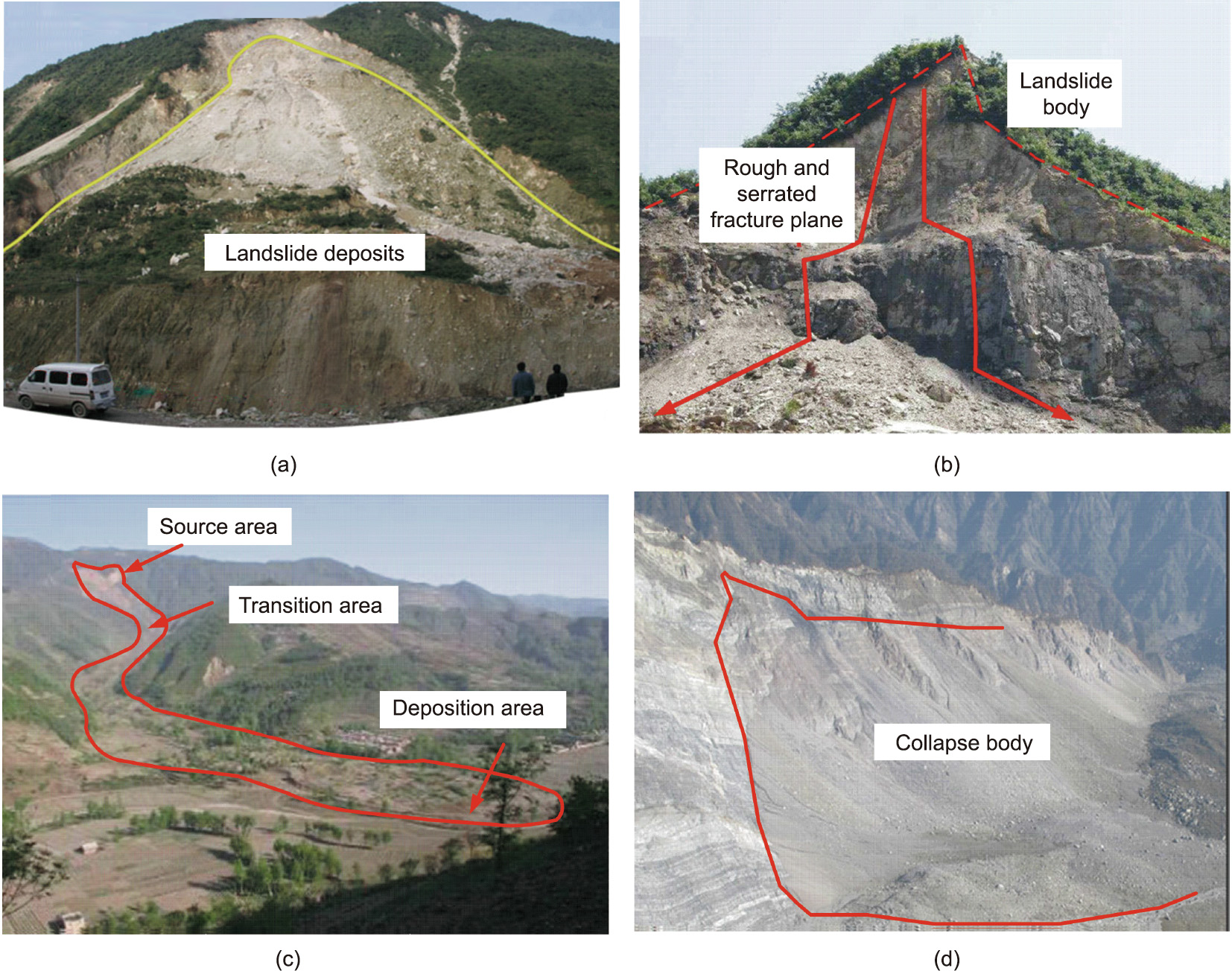
Fig. 1. Landslides induced by earthquakes. (a) Guantan landslide. Reproduced from Ref. [3] with permission. (b) A landslide at Dongjia Village Qingchuan County. Reproduced from Ref. [4] with permission. (c) Touzhai valley landslide. Reproduced from Ref. [5] with permission. (d) Daguangbao landslide. Reproduced from Ref. [6] with permission.
These studies mainly focused on either analyzing the phenomenon and the distribution of earthquake-induced landslides, or on crack models. However, these studies did not identify the mechanisms of crack initiation and propagation within rock masses under seismic loading. Crack initiation, propagation, and coalescence, combined with strength degradation induced by localized failure and deformation, are the main reasons for the failures of jointed rock slopes [14]. The cracking processes are also significantly influenced by discontinuities contained within the rock mass (e.g., natural fractures, bedding plane, faults, and joints). Opening-mode fractures are found extensively in rock masses (Fig. 2) [15–17] due to various external geological forces (e.g., deposition, river erosion, and weathering processes [18,19]). When an earthquake occurs, cracks initiate and develop in the rock mass. These damaged rock masses and slopes are prone to sliding. The earthquakes are then usually followed by a considerable number of aftershocks that usually induce several landslides [20,21].
《Fig. 2》

Fig. 2. Field observations of various flaws. (a) Pre-existing open holes contained in rock masses. Reproduced from Ref. [15] with permission. (b) Discontinuity configuration. Reproduced from Ref. [16] with permission. (c) Rock mass with deep open flaws. Reproduced from Ref. [17] with permission.
The present numerical study aimed to investigate the effect of seismic loading on crack initiation and propagation in a model containing a single flaw, based on the bonded-particle model (BPM). The BPM can not only simulate cracking and damage accumulation in rocks, but can also mimic velocity changes within rocks under seismic loading [22]. The model offers the unique ability to directly study the process of crack initiation, propagation, coalescence, stress wave propagation, seismic wave propagation, and velocity change, which generally cannot be directly measured in laboratory or field studies [23,24].
The mechanisms of crack initiation and propagation under seismic loading are different from those under quasi-static loading [25,26]. Some researchers have used the BPM to study the seismic response of different types of rock/soil slopes under seismic loading. For example, the two-dimensional (2D) BPM was used to simulate the Tsaoling landslide, triggered by the Chi-Chi earthquake, and the mechanism causing the Tsaoling landslide [27,28]. The 3D BPM was used to analyze the wave propagation in dry granular soils [29]. These studies focused on earthquake-induced landslides caused by strong earthquakes, and the results implied that the slope models failed after seismic loading was applied. However, the initiation of a small number of discrete cracks would not immediately lead to the failure of a slope because of certain external force or earthquake intensities. Further, if the force or seismic wave were repeatedly applied to the rock mass, the extension and coalescence of these initiated cracks could ultimately cause failure. In the present study, the 2D BPM was used to study the crack initiation and propagation as a result of seismic wave loading applied, repeatedly, in either the same direction or in two orthogonal directions.
《2. Methodology》
2. Methodology
《2.1. Bonded-particle model》
2.1. Bonded-particle model
The principle of the BPM has been widely introduced in other studies [30,31]; therefore, the present study will only briefly describe its features. There are two major types of BPMs available: the contact bond model and the parallel bond model. The latter can transmit both forces and moments, and is more often used for rock simulation. The parallel bond model represents the physical behavior of a cement-like substance that connects two adjacent particles. This concept can be illustrated as a set of elastic springs, uniformly distributed over a rectangular cross-section with constant normal bond stiffness and shear bond stiffness, lying on the contact plane and centered at the contact point. This set of springs acts like a beam that resists the tensile or shear forces and moments induced by particle rotation. When the force acting on a bond exceeds the normal or shear strength of the bond, the bond breaks and a micro-crack (shear or tensile) is formed (Fig. 3) [32]. The model presents different patterns of bond breakage (shear or tensile). Zhang and Wong [33,34] used a parallel BPM to study the size effect on cracking processes under compressive loading and investigated the cracking processes in specimens containing flaws under a loading rate ranging from a static to intermediate loading rate (from 0.005 to 0.600 m·s–1 ). These studies demonstrated that the BPM is capable of simulating crack initiation, propagation, and coalescence in rocks and rock-like materials under quasi-static compressive loading.
《Fig. 3》
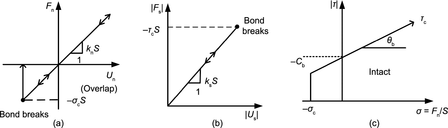
Fig. 3. Failure criterion for the parallel bond model: (a) normal force versus normal displacement; (b) shear force versus shear displacement; and (c) strength envelope. Reproduced from Ref. [32] with permission. Fn: normal force; Fs: shear force; –σc: tensile strength; Un: normal displacement; Us: shear displacement; kn: normal stiffness; ks: shear stiffness; Cb: cohesion; θb: friction angle; τc: shear strength; S: contact area between two particles.
《2.2. Wave propagation in the BPM》
2.2. Wave propagation in the BPM
A seismic wave refers to the release of accumulated energy, when an earthquake occurs, in the form of an elastic wave radiating in all directions. Owing to the heterogeneity of Earth materials, the wave propagation paths are not linear, resulting in complicated shapes after reflection and transmission. To realistically simulate crack propagation resulting from a seismic wave, it is necessary to elucidate the reflection and transmission at the specimen boundary. In the present study, unless otherwise stated, only the simplest form of the incident angle (normal incidence) was used. With respect to the finite rigidity of the underlying medium, Joyner and Chen [35] adopted a method to meet the boundary conditions exactly for a wave vertically incident on the boundary from below, which was similar to that used by Lysmer and Kuhlemeyer [36]. A vertical incident plane shear wave was assumed in the underlying elastic medium. This assumption provided an expression for the shear stress at the boundary in terms of the particle velocity of the incident wave and that on the boundary. The particle velocity ( ) and shear stress (
 ) are derived from the equations:

where 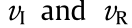 are the particle velocities of the incident and reflected waves, respectively.
  is the shear velocity in the medium, and ρ is the density of the underlying medium. When an elastic wave traveling through a given medium I reaches the boundary of another medium II, the incident wave splits into two types of waves: a reflected wave and a transmitted wave [37]. The relationship of the amplitude of the reflected wave (R) and transmitted wave (T) with that of the incident wave is given by the following equations:
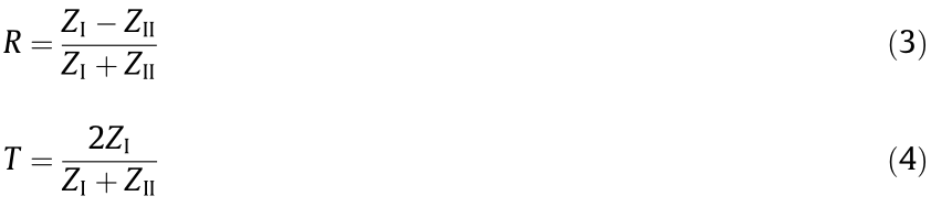
where Z is the acoustic impedance, Z = ρPw = (ρEe)1/2, Pw is the wave speed, and Ee is the modulus of elasticity. If the acoustic impedances of the two mediums are different, the transmitted and reflected waves correspond to different amplitudes and speeds (i.e., compression or rarefaction). For example, if ZII → 0, the transmitted wave has twice the magnitude of the incident wave at the same speed. The reflected wave has the same magnitude and the same speed as the incident wave. In the case of an infinitely large impedance, ZII →  there would be no transmitted wave, and the incident wave would be completely reflected back into the medium I with the opposite speed.
The preceding examples demonstrate the relationship of the amplitude and speed of the reflected and transmitted waves, with those of the incident wave under two special conditions in the BPM. Fig. 4 illustrates the plane wave propagation through a one-dimensional (1D) ‘‘bar” composed of a string of 50 particles bonded together. To absorb any incident waveform, a ‘‘quiet boundary” was set at the left end of the bar. The right end of the bar was free. In this case, ZII was zero. Eq. (2) describes the relationship between the input velocity pulse and the particle velocity on the left boundary as represented by the forced loading on the left ball. The relationship between the boundary force F and the particle velocity  is
is

where Rp is the particle radius, and  is the given velocity pulse.
《Fig. 4》
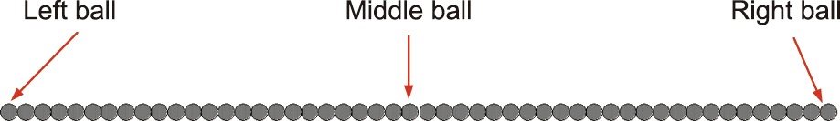
Fig. 4. Ball ‘‘bar” composed of a string of 50 particles bonded together.
The velocity pulse is given by Eq. (6):

where A is the amplitude of the pulse and  is the frequency. The ball radius of the bar was 0.5 m and the wave speed was 100 m·s–1 . The time of the given velocity pulse (t) was 0.25 s. The frequency () was 4 s–1 . The three velocity curves of the left, middle, and end ball of the bar were obtained (Fig. 5). The first and second peaks correspond to the left and middle balls along the bar, respectively. The end ball shows a peak velocity of double the input velocity, which is in response to the reflection at the free surface. The fourth peak shows the reflected wave traveling towards the left boundary, and the fifth peak shows the reflected wave passing through the left boundary. The quiet boundary then absorbed the incident energy, and no further pulses were identified [38]. In a second case, the right end was fixed at ZII →
  . The time history of the right end does not exist because there is no transmitted wave. The reflected wave has the opposite speed when compared to the incident wave (Fig. 6).
《Fig. 5》
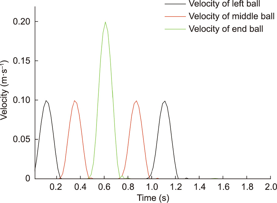
Fig. 5. Velocity histories of the free boundary: the left ball, the middle ball, and the end ball.
《Fig. 6》

Fig. 6. Velocity histories of the fixed boundary: the left ball, the middle ball, and the end ball.
The above simulations demonstrate two special conditions in the BPM, that is, a free interface and an infinitely large impedance interface. These results are in accordance with that of Jaeger et al. [37]; implying that the BPM has the capacity to simulate wave propagation in the particle model.
《2.3. Numerical model》
2.3. Numerical model
In the present study, a small rectangular specimen with the dimensions 76 mm × 152 mm was used. This dimension has been extensively employed to study crack initiation and propagation in rock mechanics [39–41]. The numerical models used in this study consisted of approximately 38 000 particles. The radius followed a uniform distribution ranging from a minimum radius of Rmin = 0.21 mm to a maximum radius of Rmax = 0.35 mm. In the BPM, the particle size had a significant effect on the macroproperties of the model. The particle size, however, did not correspond to the mineral grains within the rocks. A sufficient number of particles should be present in the model to resolve and reproduce the failure mechanisms [20]. The micro-parameters used in the model are listed in Table 1. The mechanical properties of the numerical model were compared with those obtained from laboratory tests (Table 2). The uniaxial compressive strength (UCS) of the specimen is proportional to the tensile and shear strengths of the parallel bond. Young’s modulus is proportional to the stiffness of the particle and the parallel bond. Poisson’s ratio μ is proportional to the ratio of normal stiffness to shear stiffness of particle (np/sp) and parallel bond (nb/sb). The failure model of the specimen is related to the ratio of normal strength to shear strength (i.e., σn/σs), which would determine the breakage mode of parallel bonds. However, it was not possible to directly calibrate the σn/σs ratio. Therefore, a series of uniaxial compressive tests were first conducted with different σn/σs ratios, while the other parameters were kept constant. The UCS, Young’s modulus, Poisson’s ratio, and failure mode were compared to those obtained from the experiments. Subsequently, a series of tests for different ratios of σn/σs were conducted. The crack initiation position, initiation angle, and cracking pattern were then compared to the experimental results. The micro-parameters of the BPM were obtained from this series of tests. For additional details regarding the model parameter calibration of the BPM, please refer to Zhang and Wong [31]. The specimen contained a single flaw of 12.6 mm in length and 1.3 mm in width (Fig. 7). The flaw was located at the center of the specimen, and its inclination measured from the horizontal was β = 30°, that was created by eradicating a group of particles in the center of the model. The flaw surfaces appeared rough locally (Fig. 7) because the particles in the BPM could not be divided further.
《Table 1》
Table 1 Micro-parameters of the BPM.

《Table 2》
Table 2 Comparison of the material properties of the physical experiment and numerical study [31].

PFC: particle flow code.
《Fig. 7》
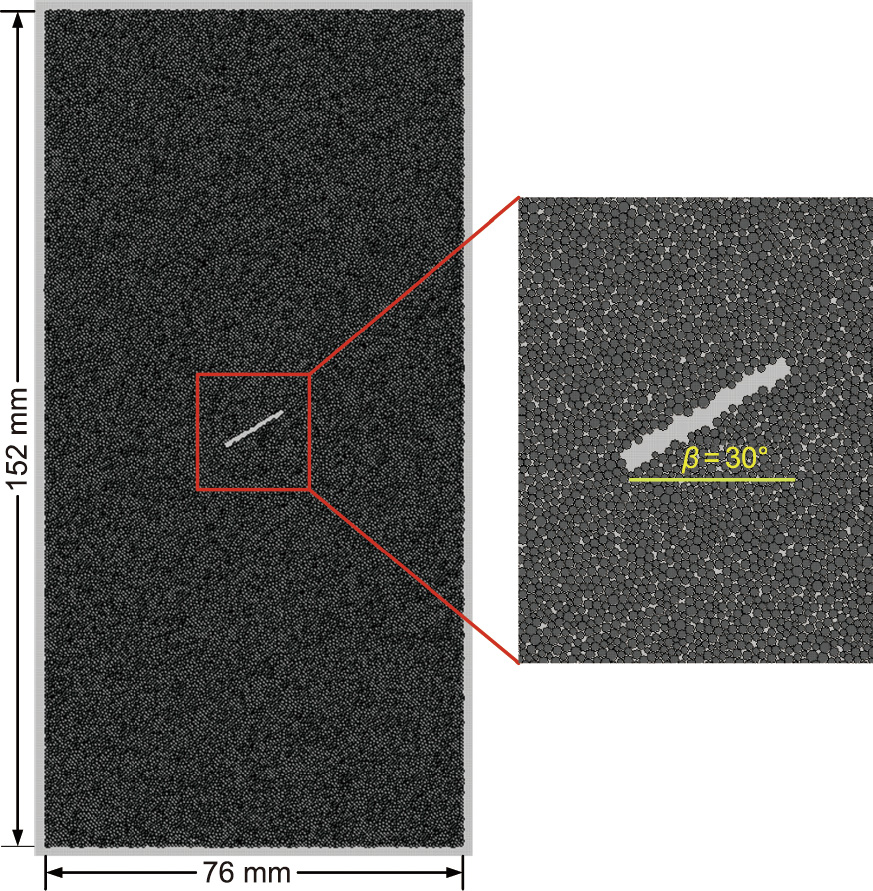
Fig. 7. Rectangular specimen (76 mm × 152 mm) containing a flaw 12.6 mm in length and 1.3 mm in width. The flaw inclination angle was β = 30°.
《2.4. Boundary conditions》
2.4. Boundary conditions
When a seismic wave is transferred from one medium to another, transmission and reflection usually occur at the interface. To prevent transmission and reflection, a viscous boundary is generally established to absorb the boundary energy, as defined by Lysmer and Kuhlemeyer [36]. However, if the size of the numerical model is very small in comparison to the wavelength of the Pwave, the reflection and transmission phenomena are not observable in the numerical model. The P-wave velocity  is defined by the following equation:
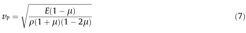
where E is Young’s modulus. In the present study, E = 6.02 GPa, μ = 0.16, ρ = 1540 kg·m–3 , and  = 2040 m·s–1 were adopted in the BPM model. The average period of the seismic wave was approximately 0.6 s. Therefore, the wavelength of the P-wave was approximately 1224 m. The length of the model was 152 mm, which accounted for 0.012% of the P-wavelength. Therefore, it was unnecessary to set a viscous boundary in the present study due to the size comparison. When the seismic wave loading was vertical, the top and bottom boundaries of the model were set as a fixed boundaries in which the velocities of the particles were equal to the given values and were not modified during cycling. The lateral boundaries were set as free boundaries in which the velocities of the particles were free to respond to the change in force during each calculation step (Fig. 8(a)). If the seismic wave loads were applied laterally, the fixed and free boundaries changed places (Fig. 8(b)).
《Fig. 8》
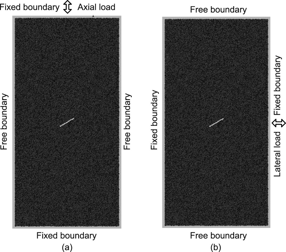
Fig. 8. (a) Boundary conditions with the seismic wave applied vertically at the top of the model: The top and bottom boundaries were set as fixed boundaries, and the lateral boundaries were set as free boundaries. (b) Boundary with the seismic wave applied laterally to the right-hand side of the model: The top and bottom boundaries were set as free boundaries, and lateral boundaries were set as fixed boundaries.
《2.5. Seismic loading》
2.5. Seismic loading
The seismic wave was applied at the top of the model and then applied to the right-hand side of the model as the P-wave velocity. In addition to monitoring the particle velocities of the model, crack initiation and propagation were observed during the loading process. The seismic wave of the Kobe earthquake that occurred on January 17, 1995, with a magnitude of 7.3 and duration of 21 s, was used as the input waveform. Figs. 9 and 10 show the velocity (maximum –90 cm·s–1 ) and acceleration (maximum 801.63 cm·s–2 ) of the input waveform. The particle flow code in two dimensions (PFC2D) user manual [38] recommends a compression test loading rate of 0.02 m·s–1 . The manual also suggests that the loading rate must be sufficiently slow to ensure that the specimen retains a quasi-static equilibrium. Zhang and Wong [33] recommended loading rates for uniaxial compression tests and Brazilian tests of 0.02 and 0.01 m·s–1 , respectively. They also advised that should the loading rate exceeded 0.08 m·s–1 ; the excessive energy would be converted to the kinetic energy. Therefore, to ensure that the specimen maintained a quasi-static equilibrium, the loading rate of the input seismic wave used was an order of magnitude less than that of the Kobe earthquake wave. The velocity of the input waveform was therefore predominantly less than 0.08 m·s–1 (maximum 0.09 m·s–1 ). The calculation in the BPM was based on Newton’s second law. To ensure that the solution produced by the model was stable, the time step (Dt) in each calculation cycle did not exceed a critical time step that depended on the stiffness, density, and geometry of the particles. In fact, the time step in each calculation cycle was set to be infinitely small at approximately 10–8 s, for the present model, so that one step in the BPM corresponded to a physical time of 10–8 s. The loading rate of 0.08 m·s–1 was translated into 8 × 10⁻⁷ mm per step, which indicated that it would require more than 1 000 000 steps to move 1 mm. The loading rate in the numerical model would, however, be different from that in a physical test. This study maintains the comparable loading wave without consideration of the realistic loading rate.
《Fig. 9》

Fig. 9. Velocity waveform of the input seismic wave. The duration and maximum velocity were 21 s and –90 cm·s–1 , respectively.
《Fig. 10》

Fig. 10. Acceleration waveform of the input seismic wave. The duration and maximum acceleration were 21 s and 801.63 cm·s–2 , respectively.
《3. Result analysis》
3. Result analysis
《3.1. Crack propagation in the model》
3.1. Crack propagation in the model
Fig. 11(a) shows the crack initiation of the specimen under axial loading, and the yellow lines indicate tensile cracks (note that no shear cracks were observed during the test, which will be discussed in Section 4). At time step 1 644 627, a few cracks initiated from the tips of the pre-existing flaw. The direction of the crack extension was perpendicular to the loading direction of the seismic waves. As the seismic loading continued, the cracks did not propagate further because the lateral velocity and displacement were relatively small and were not forceful enough to extend the crack. Subsequently, the axial load was applied again in the axial direction (Fig. 11(b)). The form and number of cracks initiated under the first cyclic loading remained unchanged during the second loading cycle. After the first cyclic loading, the total number of cracks was 60. This number was constant during the second cyclic loading, which means that no new cracks were formed. Fig. 11(c) shows the velocity and displacement curves of the two cyclic loadings. The displacement curve was obtained from the integral transformations of the time step and input velocity wave (magenta line). Fig. 11 shows that the cracks did not develop during the second cyclic loading process. This effect is known as the Kaiser effect, which was observed for cyclic loading along a given stress path and was first discovered in 1950 by Kaiser [42]. The Kaiser effect refers to the phenomenon in which acoustic emissions are observed during the first cyclic loading but absent during subsequent cycles when the stresses were below the previous peak stress; however, they then sharply increase after the stress exceeds the previous peak stress [42].
《Fig. 11》
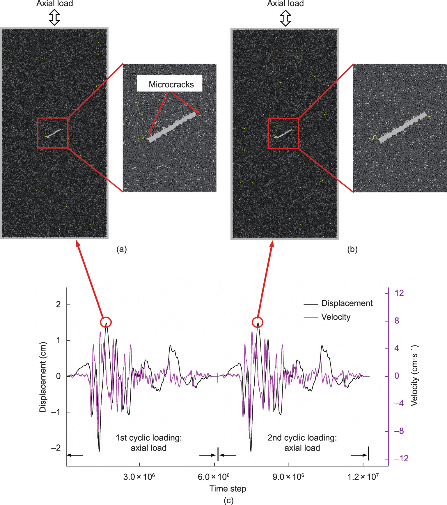
Fig. 11. (a) First cyclic loading applied on the top boundary and a few micro tensile cracks (yellow lines) initiate from the tips of the pre-existing flaw. (b) Second cyclic loading applied on the top boundary again and no new crack formed. (c) The displacement and velocity waveforms of the input seismic wave.
In contrast, after the first cyclic loading (Fig. 12(a)), the second cyclic loading was applied laterally at the same input seismic wave, time step 7 772 490, and a few new cracks appeared at the lower left and upper right-hand edges of the pre-existing fault. The direction of crack propagation was perpendicular to the lateral loading direction (Fig. 12(b)). By applying the axial load once again, time step 13 900 353, the cracks propagated in the horizontal direction ultimately splitting the specimen (Fig. 12(c)). Lavrov et al. [43] demonstrated the high sensitivity of the Kaiser effect on the rotation of the principal loading direction in a disk specimen. They proposed that the Kaiser effect completely disappeared when the rotation angle was 15° or more. Some acoustic emission experimental results [44,45] reasonably proved the directional dependency of the Kaiser effect in the orthogonal direction. When the second cyclic loading was applied in the horizontal direction, the Kaiser effect disappeared, and a few cracks were formed at the tips of the pre-existing flaw. The new cracks appearing during the second cyclic loading thus changed the stress distribution around the pre-existing flaw, resulting in a stress concentration. During the third cyclic loading, the cracks propagated along the direction of the crack initiation and ultimately divided the specimen into two parts. This phenomenon indicated that the crack propagation induced by seismic loading is dependent on the loading direction. The cracks initiated could not propagate further when seismic loading was repeatedly applied in the same direction. However, the cracks initiated would propagate further if the direction of the repeated seismic loading changed from axial to lateral. This result was useful for analyzing the crack initiation and propagation in rocks after an earthquake, and the investigation into the mechanisms of rock failure and slope instability during an aftershock.
《Fig. 12》
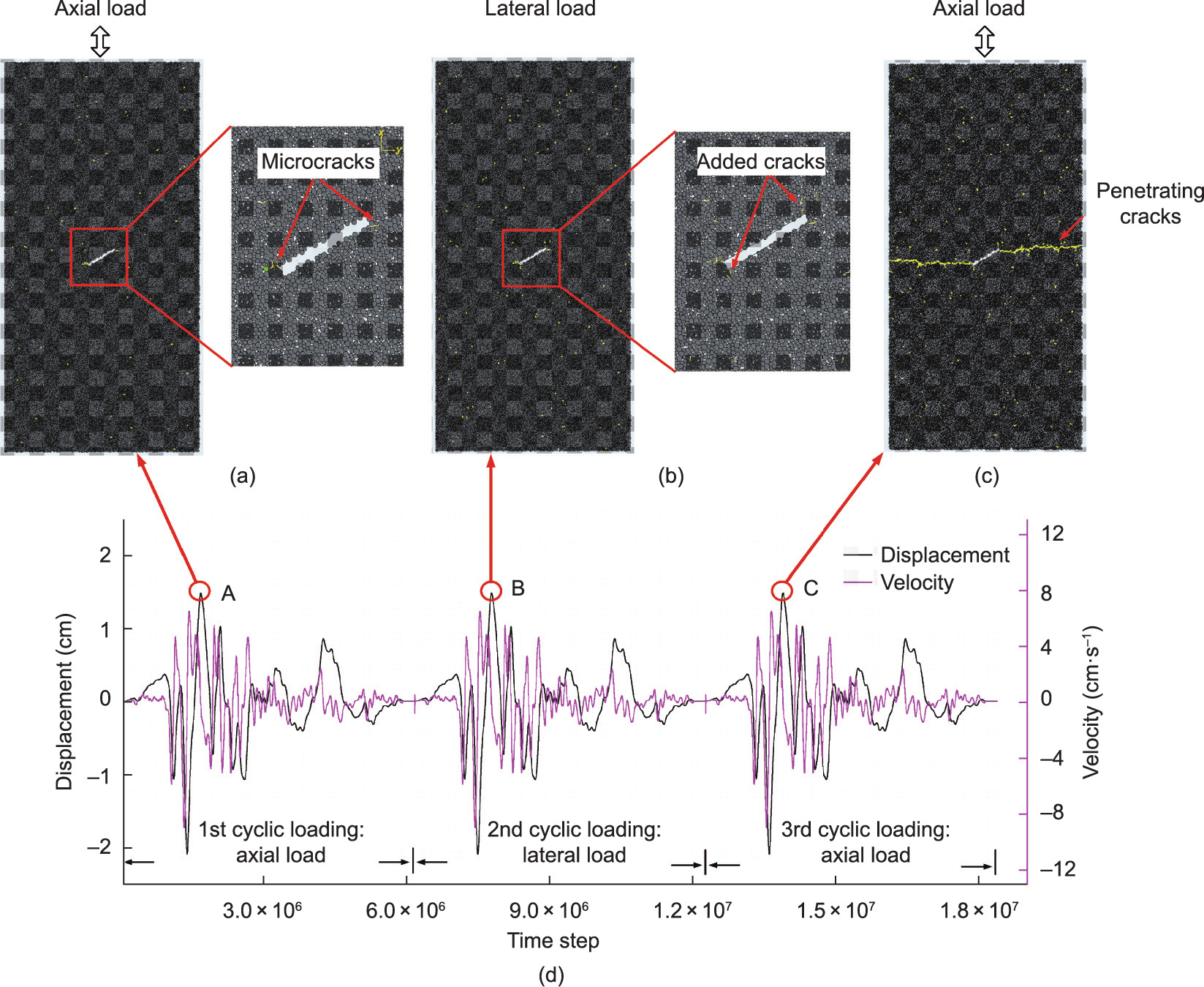
Fig. 12. (a) First cyclic loading applied on the top boundary at time step 1 644 627 exhibiting a few micro tensile cracks (yellow lines) initiated from the tips of the preexisting fault. (b) Second cyclic loading applied on the right-hand side boundary at time step 7 772 490 exhibiting a few new cracks initiated at the lower left and upper right edges of the pre-existing fault. (c) Third cyclic loading applied on the top boundary at time step 13 900 353 exhibiting cracks extending further afield forming a macro penetrating crack. (d) The displacement and velocity curves of the three cyclic loadings.
During the three cyclic loadings, crack initiation and propagation occurred at the peak tensile displacement (A, B, and C in Fig. 12(d)). A more detailed discussion on why the timing of the crack initiation was at the maximum tensile displacement rather than the maximum compressive displacement or the peak velocity is included in Section 3.2. Figs. 12(a)–(c) show that all the cracks are tensile cracks (yellow) during the loading process. If a seismic wave (large amplitude with the same waveform) is applied to an intact specimen without a pre-existing flaw, all the newly formed cracks will also be tensile cracks (Fig. 13), demonstrating that a seismic wave damaging a rock during an earthquake will do so solely through tensile failure.
《Fig. 13》
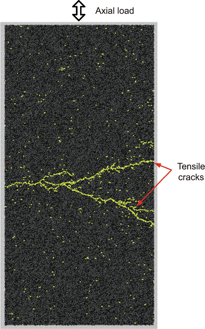
Fig. 13. A seismic wave with greater amplitude applied on the top boundary of an intact specimen. The cracks split the specimen and the crack type is tensile (yellow).
《3.2. Time of crack initiation》
3.2. Time of crack initiation
To determine the time of crack initiation, the displacement and velocity were monitored for one particle located near the crack initiation (the green ball in Fig. 12(a) with the position of x = –7.4 mm, y = –2.89 mm). Fig. 14 shows the displacement and velocity curves of the green ball under the first cyclic loading (Figs. 12(a) and (d)). The time of crack initiation (Point A in Fig. 14) does not correspond to the maximum velocity or the maximum compressive displacement (–0.15 mm); however, it corresponds to the maximum tensile displacement (0.11 mm) (in this study, the tensile displacement was positive and the compression displacement was negative). In the BPM, the maximum tensile stress or shear stress was closely related to the displacement of the particles instead of the velocity. In brief, the tensile and shear stresses were expected to reach a peak corresponding to the time of maximum displacement of the particle. In addition, the compressive strength of a rock is generally 4–25 times its tensile strength. Therefore, cracks initiate when the maximum tensile displacement occurs rather than when the maximum compression displacement occurs. It was observed that after crack initiation, the velocity of the green ball fluctuated dramatically. This fluctuation was caused by the sudden release of stress concentration around the cracks. After a few time steps, the stress was redistributed and reached a new equilibrium and the particle velocity returned to normal (Fig. 14).
《Fig. 14》

Fig. 14. Displacement and velocity curves of the green ball during the first cyclic loading (in Figs. 12(a) and (d)). The cracks are formed at the maximum tensile displacement, 0.11 mm (Point A).
《3.3. Comparison of the velocity along the axial direction in the model》
3.3. Comparison of the velocity along the axial direction in the model
Figs. 15 and 16 show the curves of the velocity versus time steps of the particles in the different locations: top boundary particle (position of x = –0.03 mm, y = 74.41 mm), 1/4 particle (position of x = –0.02 mm, y = 37.15 mm), 1/2 particle (position of x = –0.02 mm, y = 2.73 mm), and 3/4 particle (position of x = –0.02 mm, y = –37.45 mm). As shown in Fig. 16(b), to clearly observe and compare the velocity ratio at various locations, the particle velocities during the period of dramatic fluctuation were not plotted. There were no reflection or transmission phenomena during the seismic loading processes, as discussed in Section 2.3. The velocity curves of these particles were similar; however, the velocity values were different under a linear ratio (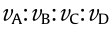 = 4:3:2:1). The strain rate was used more often than the loading rate in the physical testing. The strain rate refers to the rate of change in the strain and is presented in Zhang and Wong [33] and is denoted as
  :
:

where ε is the strain, t is the time, L is the specimen length, L0 is the original specimen length, and  is the loading rate. Because the bottom boundary was fixed during axial loading, the strain rate was uniform throughout the specimen. This implies that the velocity of a particle is determined to its location. For example, the velocity of the particle around the boundary (Point A) is twice that located in the middle area (Point C), corresponding to the specimen lengths L and L/2, respectively.
《Fig. 15》
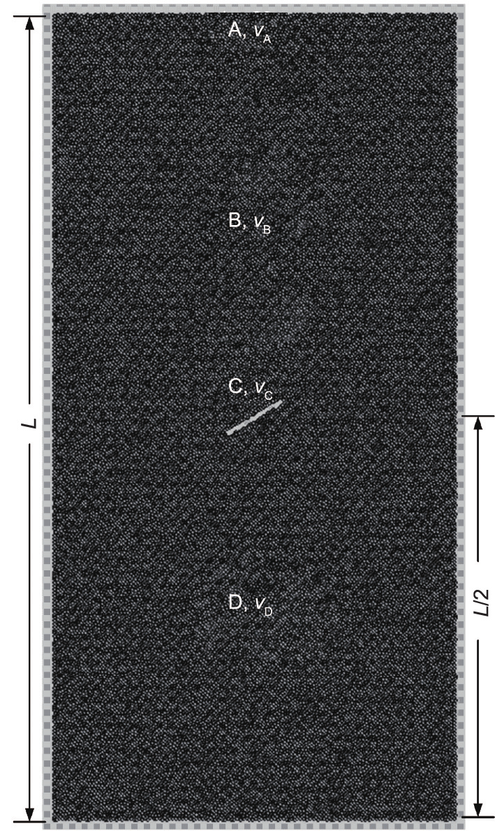
Fig. 15. Sketch of the locations of the four selected particles: A, B, C, and D. L is the specimen length.
《Fig. 16》
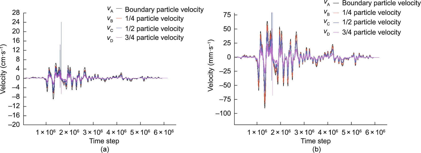
Fig. 16. Velocity curves of the four particles at different locations of the specimen: boundary particle, 1/4 particle, 1/2 particle, and 3/4 particle. The velocity curves are similar; however, the velocity values are different under a linear ratio, = 4:3:2:1; (b) is an enlarged portion of (a).
From the above discussion, it can be concluded that in the discrete particle model, the velocity distribution along the loading direction exhibits a generally linear distribution. The particle velocity in the model gradually changes, which is similar to the velocity distribution in a continuously distributed material or numerical model.
《4. Discussion》
4. Discussion
When an earthquake occurs, seismic loading acting on a rock mass in any direction can be divided into horizontal and vertical components. A rock mass is subjected to the combined effects of tension and shear. Rock mass collapse under seismic loading is a complex process that involves wave propagation, energy attenuation, crack initiation, propagation, and coalescence. For a better understanding of the relationship between the direction of seismic loading and the direction of crack initiation, some studies have been carried out based on rock fracture mechanics and seismic energy [46,47]. The results of these studies indicate that as the angle between the direction of the seismic wave input and the horizon increases from 0° to 90°, the angle of crack initiation increases from 0° to 70.5° (Fig. 17) [47]. This phenomenon is comparable to the present study, which evaluates the cracking processes in a model containing an open flaw under seismic loading.
《Fig. 17》
Fig. 17. Influence of direction of seismic wave on crack initiation. Reproduced from Ref. [47] with permission.
The present study indicates that the failure nature of cracks is tensile. This is in agreement with the observations made in some landslides [48] and laboratory tests [49] (Fig. 18). Tensile stress causes the head scarp of a landslide induced by an earthquake to be generally serrated, rough, and steep. This differs from the smooth arc-shaped scarp of a gravitational landslide caused by shear stress. Seismic loading plays a significant role in the early stages of earthquake-induced landslides. It generates tensile stress that results in tensile cracks in the rear of the slope (Fig. 19) [6]. Tensile stress plays a dominant role in landslide deformation. At the same time, seismic loading results in the fracturing of the rock mass and reduces the cohesion strength of the substrate. As cracking develops and strength decreases, landslides occur.
《Fig. 18》

Fig. 18. Tensile cracks observed in some landslides. Reproduced from Refs. [48,49] with permission.
《Fig. 19》
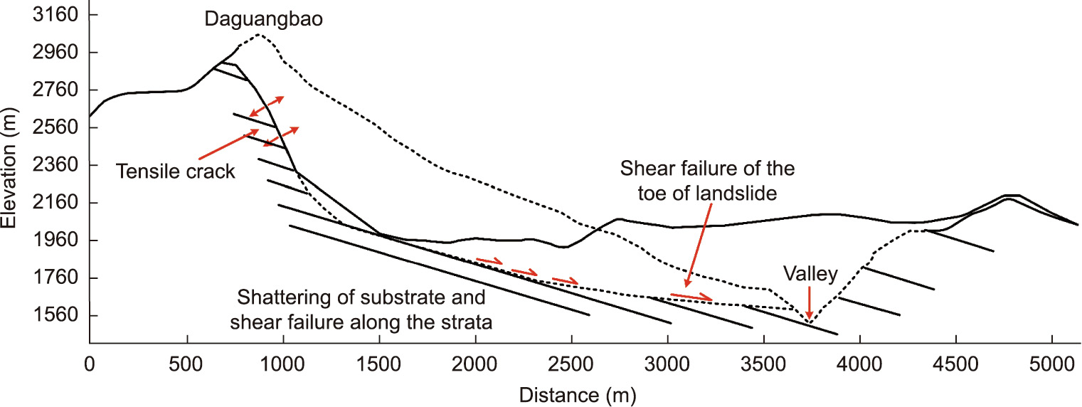
Fig. 19. Concept model of failure mechanism of a landslide. Reproduced from Ref. [6] with permission.
These findings explain why a considerable number of landslides have occurred during aftershocks. Because reflection and transmission occur within large-scale slopes and rock masses in the field, the rocks undergo the seismic loadings of aftershocks repeatedly and these are applied from different directions, which induces further propagation of the initiated cracks and failure of the rock slope. However, the present study is a simple 1D model for studying wave propagation and cracking processes. In addition, the cracking processes are also affected by the size, location, and dip angle of the pre-existing fracture, moisture content, confining stress, rock type, and other factors. Further investigations are needed to determine how seismic waves cause rock mass damage and induce landslides with regards to topics such as seismic wave propagation on a large-scale slope by considering the effects of terrain, geological conditions, topographic amplification, and on-site stress states through laboratory tests and numerical studies.
《5. Conclusions》
5. Conclusions
Based on the parallel BPM approach, the present study presents a simulation of the cracking processes under cyclic seismic loading from two orthogonal directions. The direction of crack initiation and propagation and the failure mechanism of cracks induced by seismic loading are discussed. The major conclusions are summarized as follows:
(1) During the seismic loading process, the failure of the specimen is tensile in nature.
(2) Crack initiation and propagation occur when peak tensile displacement occurs in the seismic loading sequence.
(3) If seismic loading from only the axial direction is repeatedly applied to the specimen, only a few microcracks are initiated from the pre-existing flaw tips. These microcracks do not propagate further. However, as the same seismic loading is repeatedly applied to the specimen from the axial and lateral directions, the initiated cracks propagate further, and the specimen ultimately fails.
《Acknowledgments》
Acknowledgments
The authors would like to thank the National Natural Science Foundation of China (52108382, 51978541, 41941018, and 51839009), and China Postdoctoral Science Foundation (2019M662711) for funding provided to this work.
《Compliance with ethics guidelines》
Compliance with ethics guidelines
Xiaoping Zhang, Qi Zhang, Quansheng Liu, and Ruihua Xiao declare that they have no conflict of interest or financial conflicts to disclose.


 京公网安备 11010502051620号


