《1. Introduction》

1. Introduction

The design and realization of micromanipulators and microrobots has recently become an important field of research. Potential areas of application are microsurgery, micromanufacturing, and microassembly [1]. Several micro-actuation techniques have been developed, mostly based on smart materials such as piezoelectric actuators and shape memory alloys. The most popular micro-positioning motion mechanism is the stick-slip principle [2], which is implemented using piezoelectric actuators. This principle is employed by the MINIMAN microrobot presented in Ref. [3], among other examples. These platforms are capable of a positioning accuracy of less than 200 nm, and provide velocities of up to a few mm.s⁻¹. The impact drive principle, a variant of the stick-slip principle, is employed by the 3-degree-of-freedom (3-DOF) microrobotic platform Avalon, which provides a step size of about 3 μm and speeds up to 1 mm.s⁻¹ [4]. A different motion mechanism based on piezo-tubes is utilized by the Nano Walker microrobot [5]. The first prototypes of this microrobot were capable of minimum steps on the order of 30 nm, and demonstrated a maximum linear speed of 200 mm.s⁻¹. The MiCRoN may be the most advanced example of a microrobotic platform; it employs piezoelectric actuators with an integrated micromanipulator [6].

Although piezoelectric actuators seem to be the preferred smart material for micropositioning, since they provide the required positioning resolution and actuation response, they usually suffer from complex power units that are expensive and cumbersome, and that do not easily allow for untethered operation. Small-scale piezoelectric drivers and amplifiers that can be accommodated on board are custom-made and thus do not allow for cost-effective designs [7]. Vartholomeos and Papadopoulos [8] proposed a novel, simple, and autonomous microrobot driven by two vibrating micromotors that is able to perform translational and rotational sliding with micrometer positioning accuracy and velocities up to 1.5 mm.s−1. All the components of this mechanism, including its driving units, are of low cost and readily available. Although the use of only two vibration micromotors significantly simplifies the microrobot design, it introduces nonholonomic motion constraints. During the last three decades, extensive research has been carried out on nonholonomic path planning, mostly of wheeled robots. Some examples of the research in the field are presented in Refs. [9¯14].

This paper focuses, for the first time, on the formulation and practical implementation of positioning methodologies that compensate for the nonholonomic constraints of a mobile microrobot that is driven by two vibrating direct current (DC) micromotors. More specifically, the contributions of this paper include: ① The formulation of a positioning methodology based on an open-loop approach, ② the formulation of two positioning methodologies based on a closed-loop approach, and ③ the implementation of the proposed methodologies in a prototype microrobot, and their experimental validation. The rest of the paper is structured as follows. A brief description of the microrobotic platform is presented in Section 2. In Section 3, the proposed positioning methodologies are studied. Simulation runs and experiments are presented and evaluated in Sections 4 and 5, respectively.

《2. Brief description of the microrobot》

2. Brief description of the microrobot

A brief description of the mobile microrobot is given here. For a more detailed presentation of the dynamics, design, and innovative actuation principle of the microrobot, see Ref. [8].

《2.1. Motion principle》

2.1. Motion principle

A simplified 1-DOF mobile platform of mass M is used, whose motion mechanism employs an eccentric mass m, rotated by a platform-mounted motor O, shown in Figure 1. One cycle of operation is completed when the mass m has described an angle of 360°.

《Fig. 1》

Fig.1 Simplified 1-DOF platform with eccentric rotating mass m. In the figure, m is pointing at the center of mass of the eccentric part, which has an offset r with respect to the axis of rotation.

Gravitational and centripetal forces exerted on the rotating mass are resolved along the Y- and Z-axes to yield:

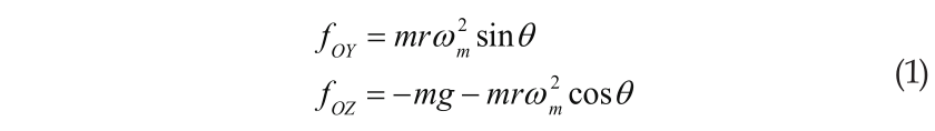
where ω_m is the actuation (motor) speed; θ is the rotation angle of the eccentric mass; g is the acceleration of gravity; and r is the eccentricity of the rotating mass m. Above a critical value of actuation speed ω_critical, actuation forces overcome frictional forces and motion is induced. The equations of motion of the simplified platform are numerically simulated to yield the results depicted in Figure 2.

《Fig. 2》

Fig.2 Simulation results for the motion of a 1-DOF example.

It is clear that for a counterclockwise rotation of the eccentric mass m, the platform exhibits a net displacement toward the positive Y-axis. It has been shown analytically that the motion step the platform exhibits over a cycle of operation can be made arbitrarily small depending on the actuation speed ω [8]. In practice, the motion resolution is limited by the electronic driving modules and by the unknown non-uniform distribution of the coefficient of friction μ along the surface of the planar motion.

《2.2. Platform dynamics》

2.2. Platform dynamics

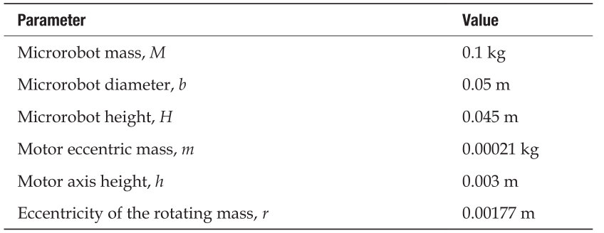
The actuation principle mentioned above was employed in the design and implementation of a 2-DOF microrobot, as shown in Figure 3. A needle is mounted on the microrobot, and its tip represents the end-effector. Some physical parameters of the microrobot are presented in Table 1.

《Fig. 3》

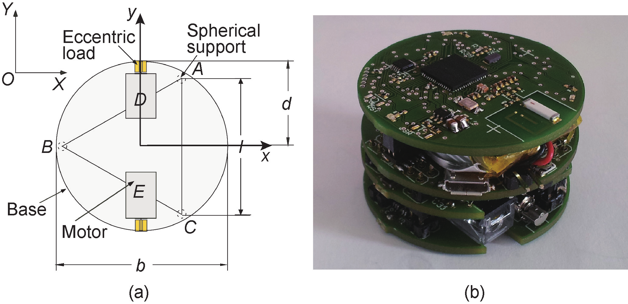
Fig.3 (a) Base design; (b) prototype.

《Tab.1》

Tab.1 Physical parameters of the microrobot.

The platform dynamics are presented in a compact matrix form using the Newton-Euler equations:

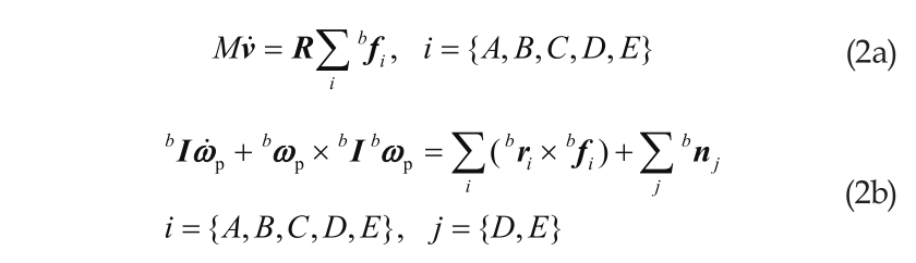
where b is the body fixed frame; R is the rotation matrix between frame b and the inertial frame O; ω_p is the platform angular velocity; ^bI is its inertia matrix; and v = [d x/d t, d y/d t, d z/d t]^T is its center of mass velocity with respect to the inertial frame O. The vector f_i^b includes the reaction forces at the three contact points of the platform, and the actuation forces generated by the two DC vibrating motors, i = { A, B, C, D, E}. The actuation moments exerted by the motors are denoted by n_j^b, j = { D, E}. During the analysis, the equations are simplified as the microrobot undergoes a planar motion.

The actuation forces generated by a motor when its eccentric load rotates are given by the following equations:

where φ_j is the angle of the motor axis with respect to the forward-looking main diameter of the platform X-axis in Figure 3(a). In the case of two motors, the angles φ_j∈{90°,–90°}.

《3. Positioning methodologies》

3. Positioning methodologies

Simulation runs and experiments regarding the basic motion capabilities of the platform indicated that the microrobotic platform is capable of moving forward and backward, as well as diagonally; and that it can rotate in both clockwise and anticlockwise directions [15]. The possible motions of the platform are presented in Figure 4. In this figure, ω D and ω E are the rotational speeds of the D and E actuators, while the superscripts “+” and “–” indicate the positive and negative speed, respectively. Unlike mobile robots driven by wheels, here, when only one micromotor is driven, the microrobotic platform moves diagonally and does not rotate (Figure 4). This is a consequence of the interaction between the actuation forces from the vibrating micromotors and the frictional forces acting on the platform.

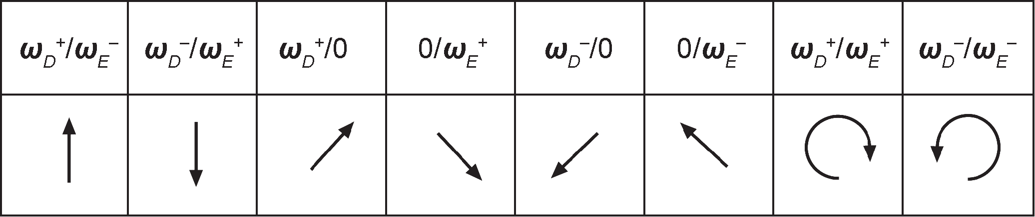
Fig.4 Possible directions of the motion of the microrobotic platform.

Moreover, due to the nonholonomic constraints, it is impossible for the platform to move parallel to the Y-axis connecting the two motors. This would be a limitation during a micromanipulation procedure, because the motion of the platform in the forward direction results in a small parasitic sideways deviation. More specifically, because of unmodeled dynamics, the platform may deviate toward the sidewise direction from its straightforward motion by a small amount, Δ y. Since the platform is incapable of moving in the sidewise direction so as to correct this parasitic effect, a method of performing such a positioning correction must be developed. A benefit of such a method would be to increase the flexibility of the motion of the platform, as it would be possible to execute more complex trajectories, instead of point-to-point motions.

Next, we focus on the derivation of methodologies for the achievement of a net sidewise displacement (Δ y) of the platform, by the execution of a complex (composite) motion. Toward this goal, we examine two different approaches: First, we achieve net displacement using an open-loop approach; and second, we develop two distinct algorithms for a closed-loop approach.

《3.1. Open-loop approach》

3.1. Open-loop approach

An open-loop approach can yield corrections without additional hardware or complexity, and is thus studied first. This approach is developed by studying the motion of the microrobotic platform. The first step is to derive a sequence of possible motions that in theory should have as a result a net sidewise displacement of the robot. After experimentation, we concluded that the most effective method is executing a V-shaped motion, divided into two symmetrical stages. The first part of the motion is achieved when the left motor rotates in the positive direction. In the second half of the motion, only the right motor rotates with positive angular velocity, as shown in Figure 5(a).

《Fig. 5》

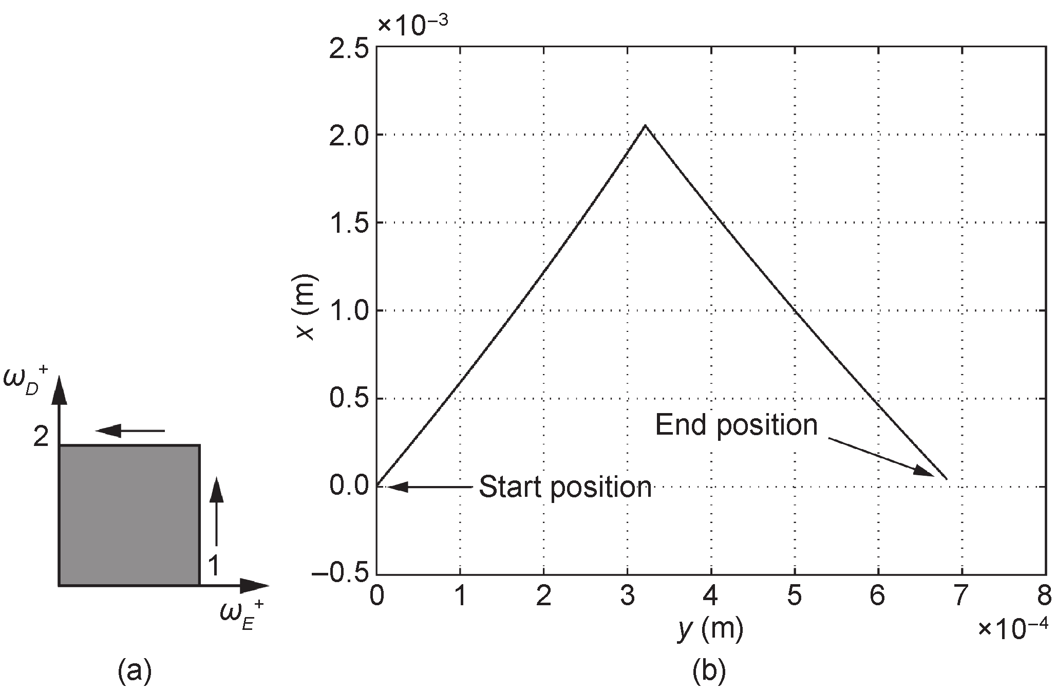
Fig.5 (a) Angular velocities succession for the sidewise displacement; (b) simulated resulting motion of the platform.

Next, a function that correlates the sidewise net displacement with the angular velocity of the motors and the duration of their operation was developed. To this end, a sufficiently large number of simulations were carried out, where different sets of angular velocities of the actuators and their operation time were the inputs of the model, and the output was the net displacement. The angular velocities that were used as input to the model were in the 800–1200 rad.s⁻¹ (7640–11 460 r.min⁻¹) range, with increments of 50 rad.s⁻¹.

The selected range guarantees that the resulting actuation forces are sufficient to overcome the frictional forces, and that no loss of static equilibrium along the vertical axis and tip of the platform can occur [8]. As we were interested in small side displacements of the order of 100¯900 μm, the duration of the motion, that is, the operation time for each motor, was chosen accordingly. Using the data provided by the simulations, the 3D graphic of Figure 6 was obtained.

《Fig. 6》

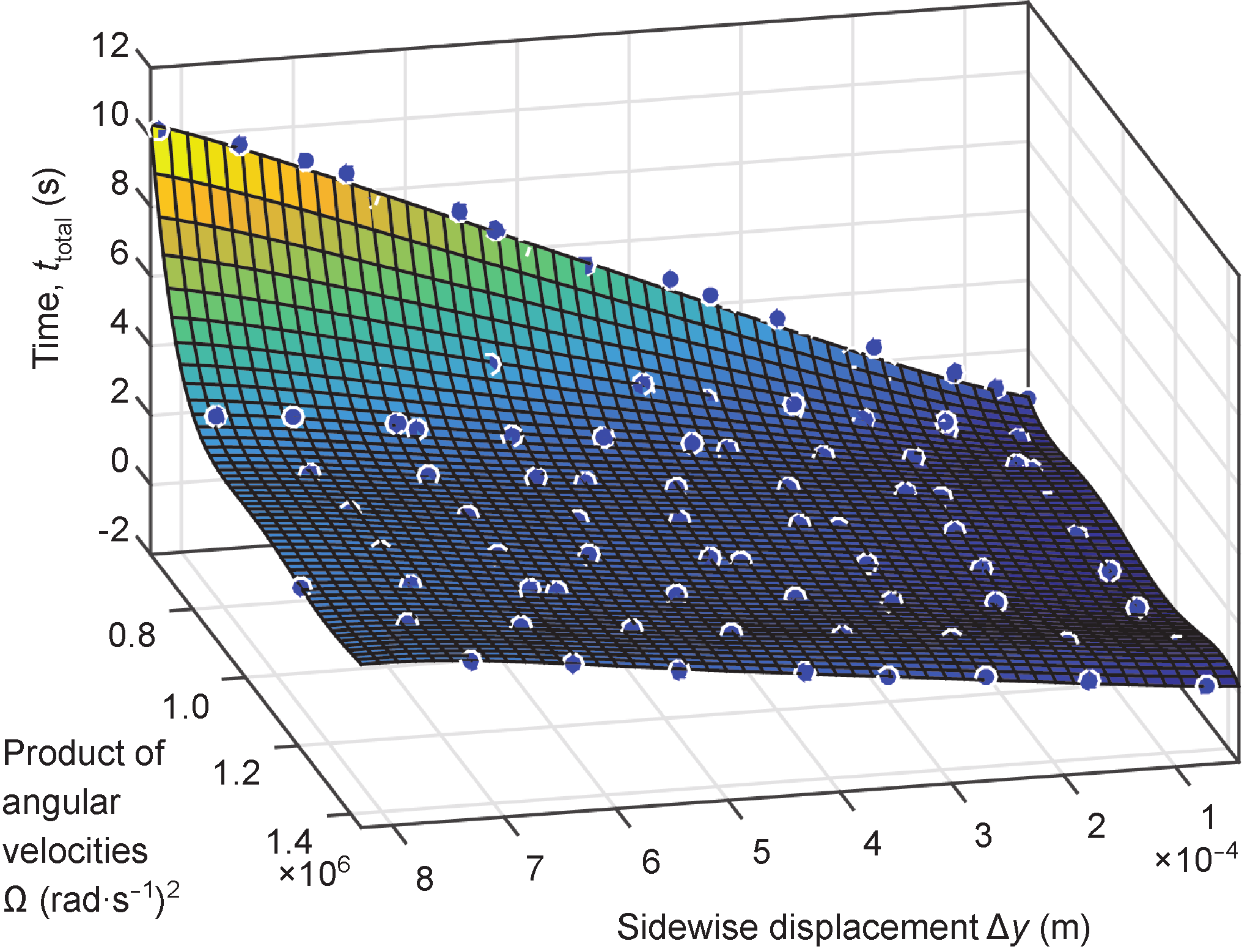
Fig.6 Polynomial fit for the open-loop simulation results.

In Figure 6, the duration of the motion, t_total (in “s”), is given as a function of the net desired sidewise displacement, Δ y (in “m”), and a measure of the angular velocities, equal to the product of the two motor angular velocities, Ω (in “(rad.s⁻¹)²”), corresponding to the gray area in the angular velocity succession given in Figure 5(a).

As expected, as the angular velocities increase, the time required for the sideways displacement decreases. Also, as this displacement increases, it takes more time to achieve it. By a polynomial fit to the data, we obtain the following function:

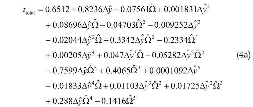
that provides t_total, with the input variables being:

where the superscripts “mean” and “std” indicate the mean value and the standard deviation, respectively ( ∆y_mean = 1.815 × 10⁻⁴ m, D y_std = 2.509 × 10⁻⁴ m, Ω_mean = 9.57 × 10⁵ (rad.s⁻¹)², and Ω_std = 2.617 × 10⁵ (rad.s⁻¹)²).

《3.2. Closed-loop approach》

3.2. Closed-loop approach

The open-loop approach is a straightforward method to achieve the desired motion. However, both the simulation results and the experiments reveal a limitation in the implementation of this method: the parasitic displacement that appears in the X- and Y-axes, due to unmodeled dynamics. As a result, two distinct algorithmic methodologies for the design of a closed-loop approach are developed. Both methodologies are based on the existence of a system that can track the motion of the end-effector of the microrobot, and that can control, during operation, the angular speed of the micromotors. In our setup, a microscope equipped with a video camera tracks the motion of a needle tip that is attached to the microrobot, as shown in Figure 7. Each image frame is transmitted to a personal computer, and processed immediately by an image-processing algorithm. According to the extracted position of the needle tip, the desired angular velocity of each micromotor is sent to the microrobot processing unit via a wireless connection.

《Fig. 7》

Fig.7 Microrobot under the microscope.

3.2.1. Algorithm closed-loop 1 (CL1)

The developed algorithm is divided into two parts. The first part includes a V-shaped motion, shown in Figure 8. For the first half of the total sidewise displacement, the platform moves diagonally with only the left motor positively rotating. When the robot reaches half the desired total sidewise displacement (point B in Figure 8), the right motor starts to operate solely, also positively rotating, until the robot reaches the desired sidewise displacement within the error limitations defined by the user (point E in Figure 8). At the end of this part of the motion, and if there is a parasitic displacement along the X-axis—for example, if the robot tip reaches point D or C instead of E, as detected by the microscope—the robot is set to move forward or backward, depending on whether the parasitic displacement is positive or negative. Figure 8 depicts this procedure.

《Fig. 8》

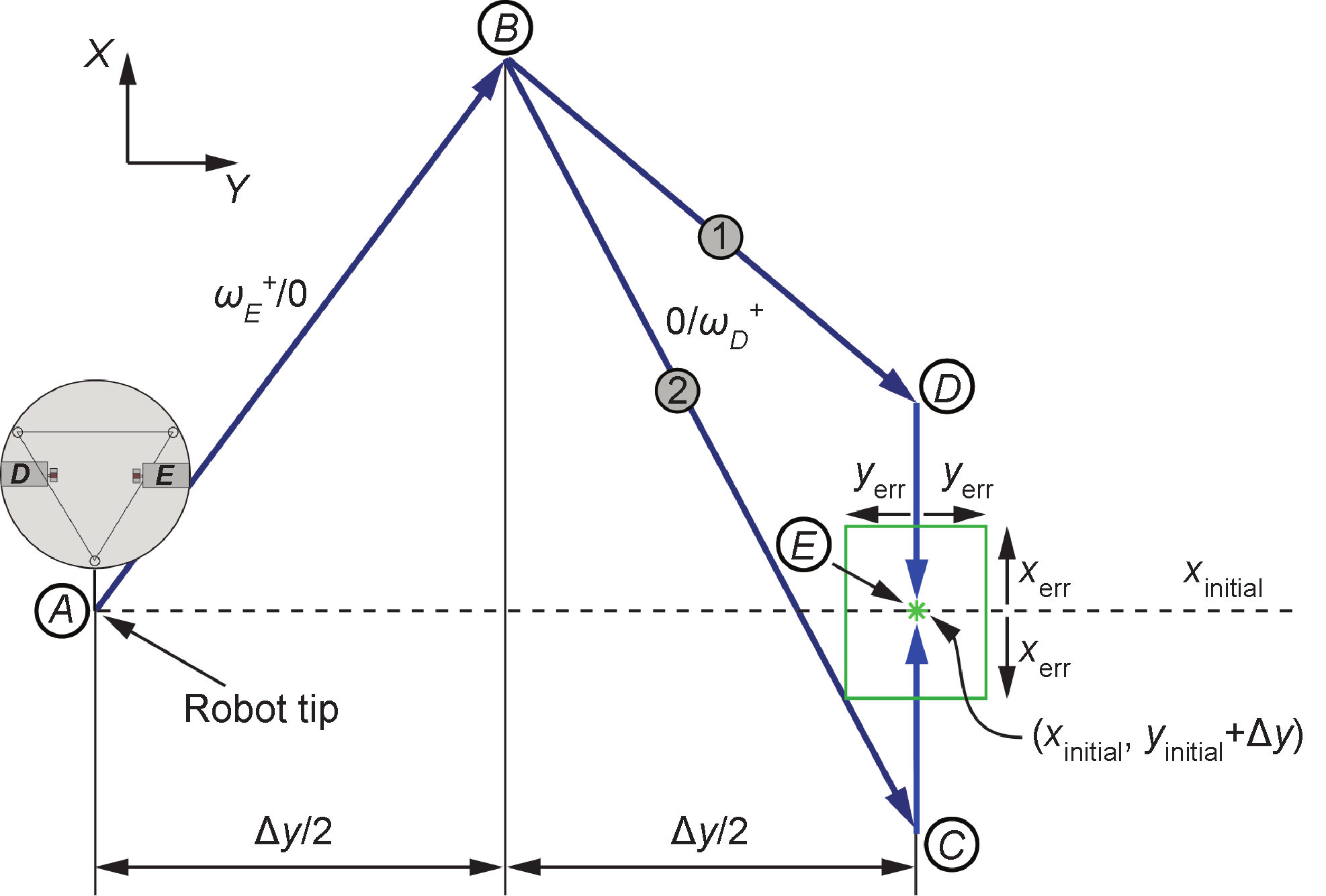
Fig.8 Schematic description of the CL1 algorithm.

Therefore, this method uses a quick single step to achieve a sidewise displacement, followed by an additional correction of the parasitic displacement from the initial X-axis. For this positioning methodology, the total duration of the motion is not predefined, but is a function of the magnitude of the desired sidewise displacement and of the needed position correction parallel to the X-axis of the robot.

3.2.2. Algorithm closed-loop 2 (CL2)

The main difference between the CL1 and CL2 approaches is the fact that in the latter, certain restrictions concerning the X-axis motion of the robot are imposed. The net sidewise displacement is no longer achieved in one step (V motion), but in multiple V cycles, depending on the total sidewise displacement and the tolerance on both axes. However, the platform is constrained to move only along the positive X-axis (or only along the negative X-axis).

More specifically, for the first half of the total sidewise displacement, the left motor is in operation, rotating in the positive direction and causing the platform to move diagonally. As soon as the robot reaches half the desired sidewise displacement, point B in Figure 9, the right motor starts to operate solely and the platform moves diagonally toward the target, point E in Figure 9. However, unlike the first algorithm, the platform is not commanded to continue until it reaches the desired Y displacement. As soon as the platform approaches the initial X-axis within an error tolerance xerr defined by the user, point C in Figure 9, it recalculates the new displacement needed to achieve the initial goal, and executes a similar V-shaped motion toward the predefined displacement, point E. This procedure is repeated until the platform has achieved the desired displacement within the user-defined specifications, by conducting a number of individual V-shaped motions each time in the direction of the desired preset sidewise displacement. Figure 9 illustrates an example of this procedure.

《Fig. 9》

Fig.9 Schematic description of the CL2 algorithm.

A feature of this methodology is that the motion of the platform is restricted only on the positive (or negative) X-axis. This can be most beneficial during a cell micromanipulation, because it can prevent damaging a cell by over-penetrating it with the needle at any point. In this approach, the total duration of the motion is also not predefined, but depends on the magnitude of the net displacement and the tolerances set by the user.

《4. Simulation results》

4. Simulation results

In the simulation runs, the goal was to achieve a desired sidewise displacement, with preset angular velocities of the motors, by following the algorithms described previously. All simulation runs were implemented with a fixed integration step size of 0.00001 s.

《4.1. Open-loop approach》

4.1. Open-loop approach

Suppose that a net sidewise displacement of ∆y = 600 μm is required for the correction of the parasitic displacement of the platform while it is moving forward; and that we wish to achieve this displacement with the angular velocities of the actuators being 1050 rad.s⁻¹, that is, Ω = 1050² (rad.s⁻¹)². Inserting these parameters into Eq. (4), and by taking into account that the ∆y and Ω coefficients are normalized as described above, we calculate that the total duration of the motion is about t_total = 2.0095 s. This duration means that the left motor will operate for 1.00475 s, and the right motor will operate for the other 1.00475 s, as shown in Figure 10. As can be inferred from Figure 10, the platform managed to achieve a sidewise displacement close enough to the desired 600 μm. The positioning error is 27.71 μm in the X-axis, and 51.67 μm in the Y-axis (8.6% error).

《Fig. 10》

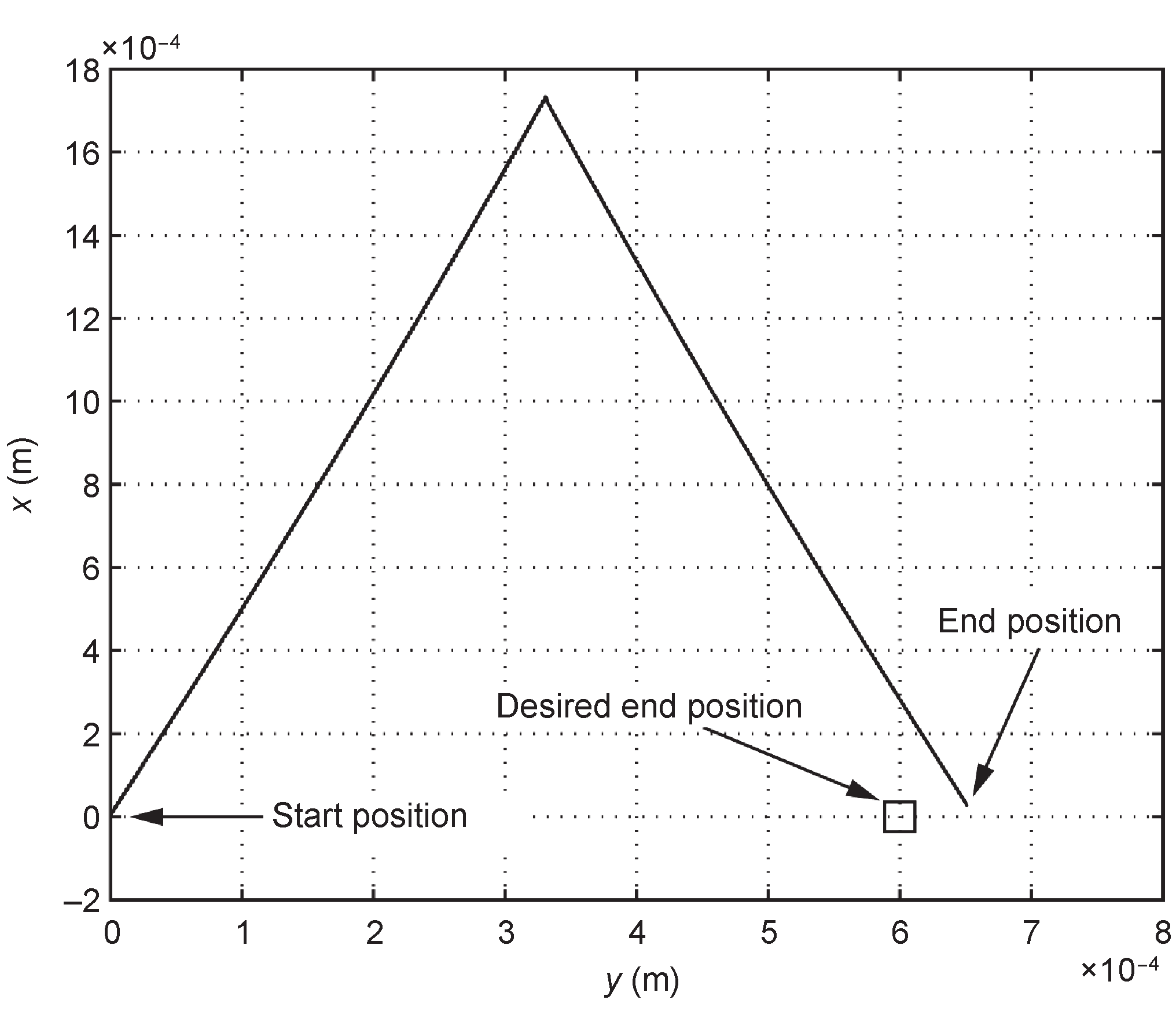
Fig.10 Path of the microrobotic platform in the open-loop approach.

《4.2. Closed-loop approach》

4.2. Closed-loop approach

In the CL2 algorithmic approach, the platform is expected to execute a number of V-shaped motions until the final point is reached. The input variables of the simulation model include the total sidewise displacement, the angular velocities, and the user-defined error tolerances. Figure 11 shows simulation results for a net sidewise displacement of 400 μm. The actuators are set to rotate at 800 rad.s⁻¹, while the tolerance of both the final y and x positions in relation to the desired ∆y and initial x respectively are set to be 10 μm. Figure 11 illustrates the path of the microrobotic platform.

The total duration of the motion was 5.225 s, in part because the sidewise displacement was large in magnitude, but also because the platform according to the algorithm performed three distinct V-shaped motions toward the achievement of the final ∆y. As can be seen from the simulation results, although the platform is constrained not to move in a negative x direction, it does move slightly toward negative x due to its dynamics, without any serious implications on the results. At the end of the motion, the platform has successfully landed inside the specified area.

《Fig. 11》

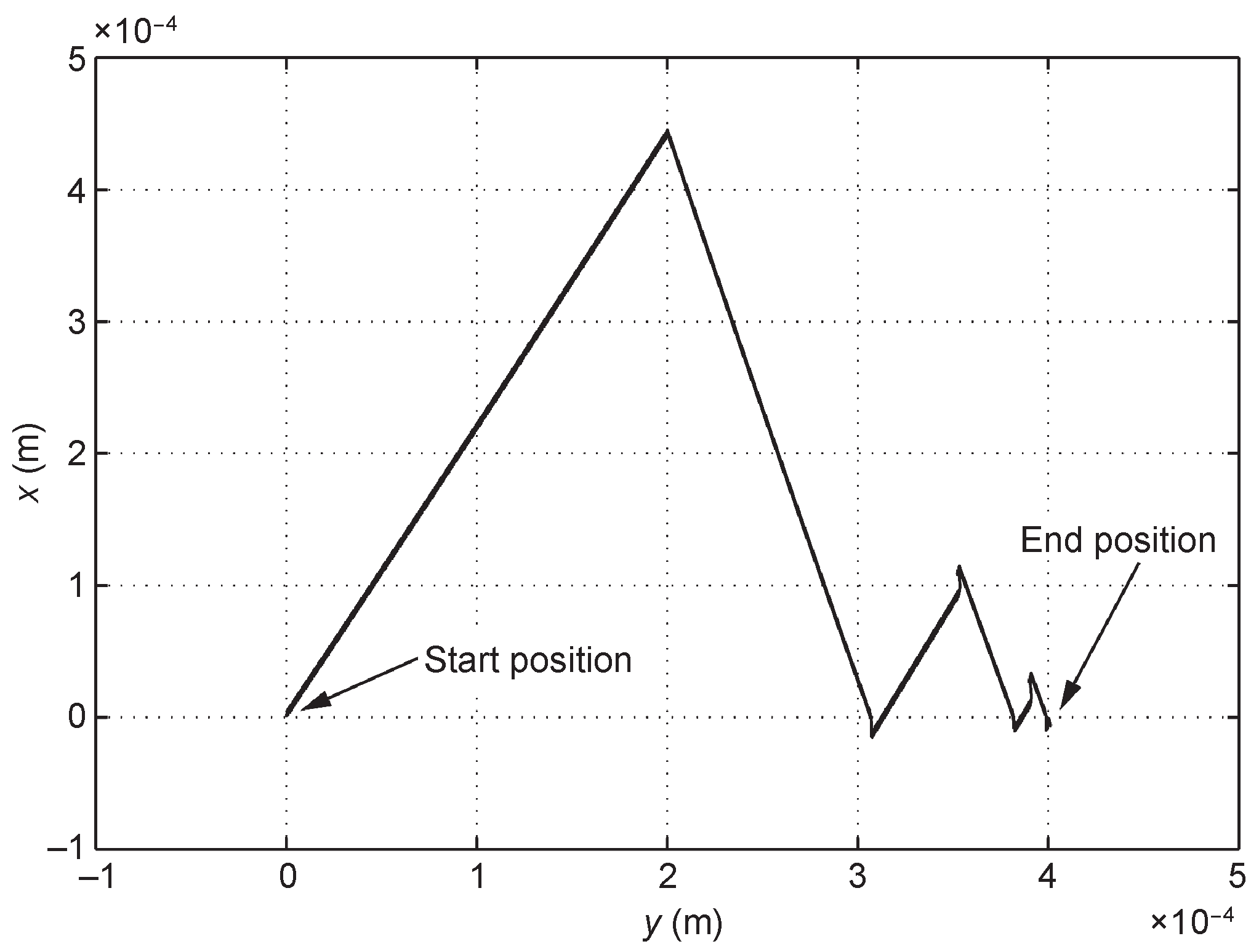
Fig.11 Path of the microrobotic platform in the closed-loop approach.

《5. Experiments》

5. Experiments

In this section, the results from experiments are given and discussed. Three experimental trials are presented. The first uses the methodology that realizes the open-loop approach, and the next two experiments use the closed-loop methodologies, CL1 and CL2.

《5.1. Open-loop approach》

5.1. Open-loop approach

In this experiment, the robotic platform executes a V-shaped step, as described in Section 3. During the first phase of the step, the left motor rotates in the positive direction. In the second half of the motion, only the right motor rotates with positive angular velocity. This specific sequence of motions results in the desired net displacement of the tip of the robotic platform toward the right of the platform, as illustrated in Figure 12.

《Fig. 12》

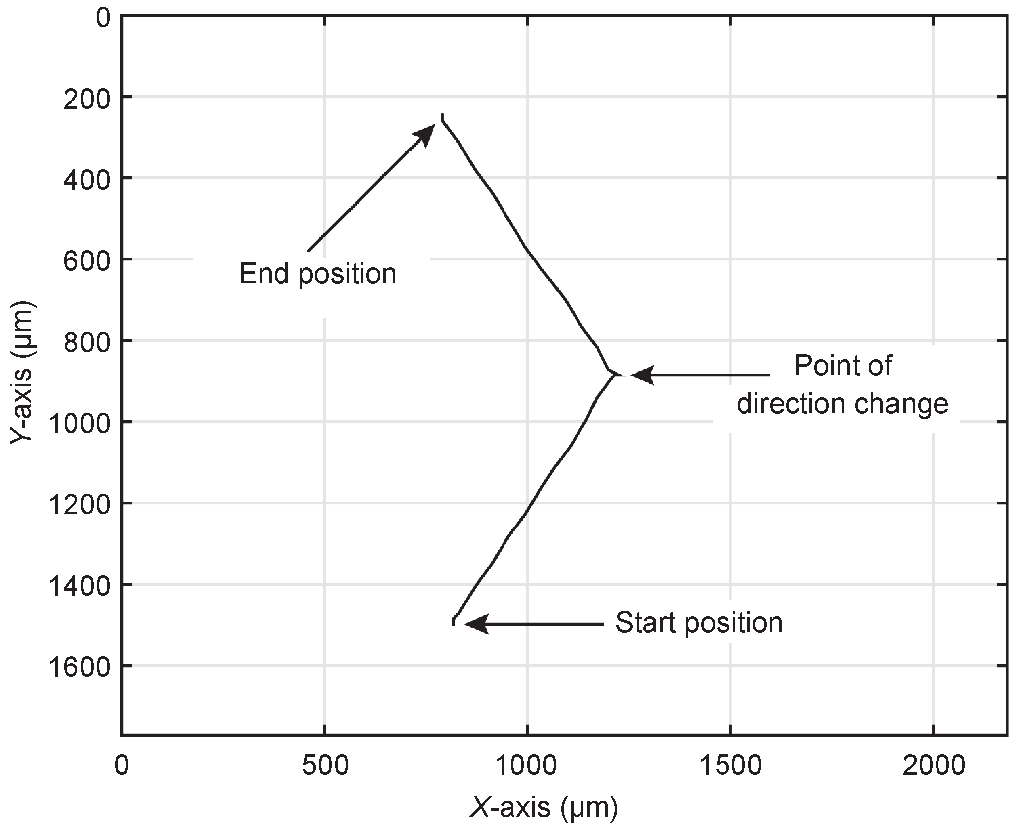
Fig.12 End-effector path using the open-loop approach.

In Figure 13, the trajectories of the microrobot along the X- and Y-axes are depicted. It is shown that each step lasts for 2 s, and results in a displacement of 1250 μm along the Y-axis.

《Fig. 13》

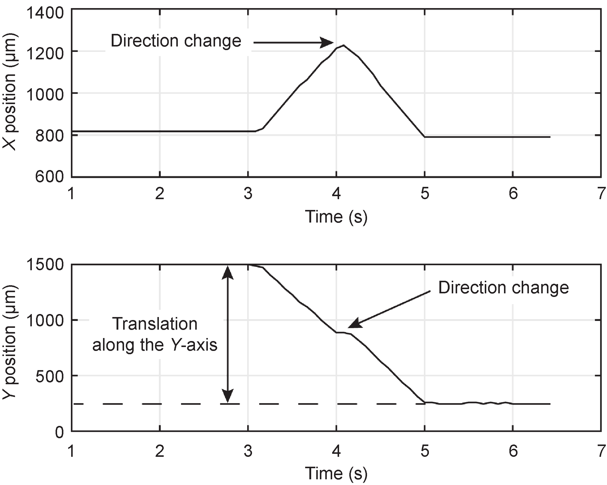
Fig.13 End-effector trajectories along the X- and Y-axes using the open-loop approach.

However, there is a total parasitic motion along the X-axis of about 50 μm. Such an undesired motion can be corrected using the methodologies of the closed-loop approach, which is presented next.

《5.2. Closed-loop approach》

5.2. Closed-loop approach

In the next experiment, the microrobotic platform moves following the CL1 methodology of the closed-loop approach, as described in Section 3. The motion of the microrobotic platform is captured by a videomicroscope, using a Marlin F146B camera from Allied Vision Technologies (Figure 7). The position is extracted on-line using an image-processing algorithm implemented in Matlab, and fed to the closed-loop system at a frequency of 12 Hz.

The start position of the tip of the platform is at x_start = 1071 μm, y_start = 550 μm, and the new desired position is x_des = 1071 μm, y_des = 65 μm. Figure 14 illustrates the experimentation results. This figure shows that, in accordance with the CL1 algorithm (Figure 8), the platform executes a V-shaped motion during the first phase until it reaches the desired ydes position. Since there is a parasitic displacement along the X-axis, the robot is set to move forward until it reaches the desired xdes position. The duration of this motion is 3.664 s. The positioning error is 35 μm in the Y-axis (7.2% error), and 6 μm in the X-axis, which represents a great improvement over the open-loop approach. The error in the Y-axis is mainly due to the parasitic displacement of the platform that occurs in the forward motion. Applying a closed-loop trajectory control algorithm can reduce this error further, with the expense of increased processing requirements.

The last experiment presents results from applying the CL2 closed-loop methodology. The location of the robot is again provided by the videomicroscope. The start position of the tip of the platform is at x_start = 750 μm, y_start = 1080 μm, and the new desired position is x_des = 750 μm, y_des = 280 μm. Figure 15 depicts the obtained results, and shows that the desired end point is reached after two consecutive V-shaped motions. The positioning error is 4 μm in the X-axis, and 13 μm in the Y-axis (1.6% error), which suggests that the CL2 closed-loop methodology offers better positioning results than the CL1 methodology.

《6. Conclusions》

6. Conclusions

This paper presented the formulation and practical implementation of positioning methodologies that compensate for nonholonomic constraints of a mobile microrobot that is driven by two vibrating DC micromotors. The methodologies are based on open-loop and closed-loop approaches, and result in a net sidewise displacement of the microrobotic platform. This displacement is achieved by the execution of a number of repeating steps that depend on the desired displacement, the speed of the micromotors, and the elapsed time. Simulation results and experiments were presented that demonstrate the performance of the proposed methodologies. The results indicate that the closed-loop approaches are much better than the open-loop approach, and that the CL2 closed-loop methodology shows a better performance than the CL1 methodology.

《Fig. 14》

Fig.14 End-effector path, and trajectory along the X- and Y-axes using the CL1 methodology of the closed-loop approach.

《Fig. 15》

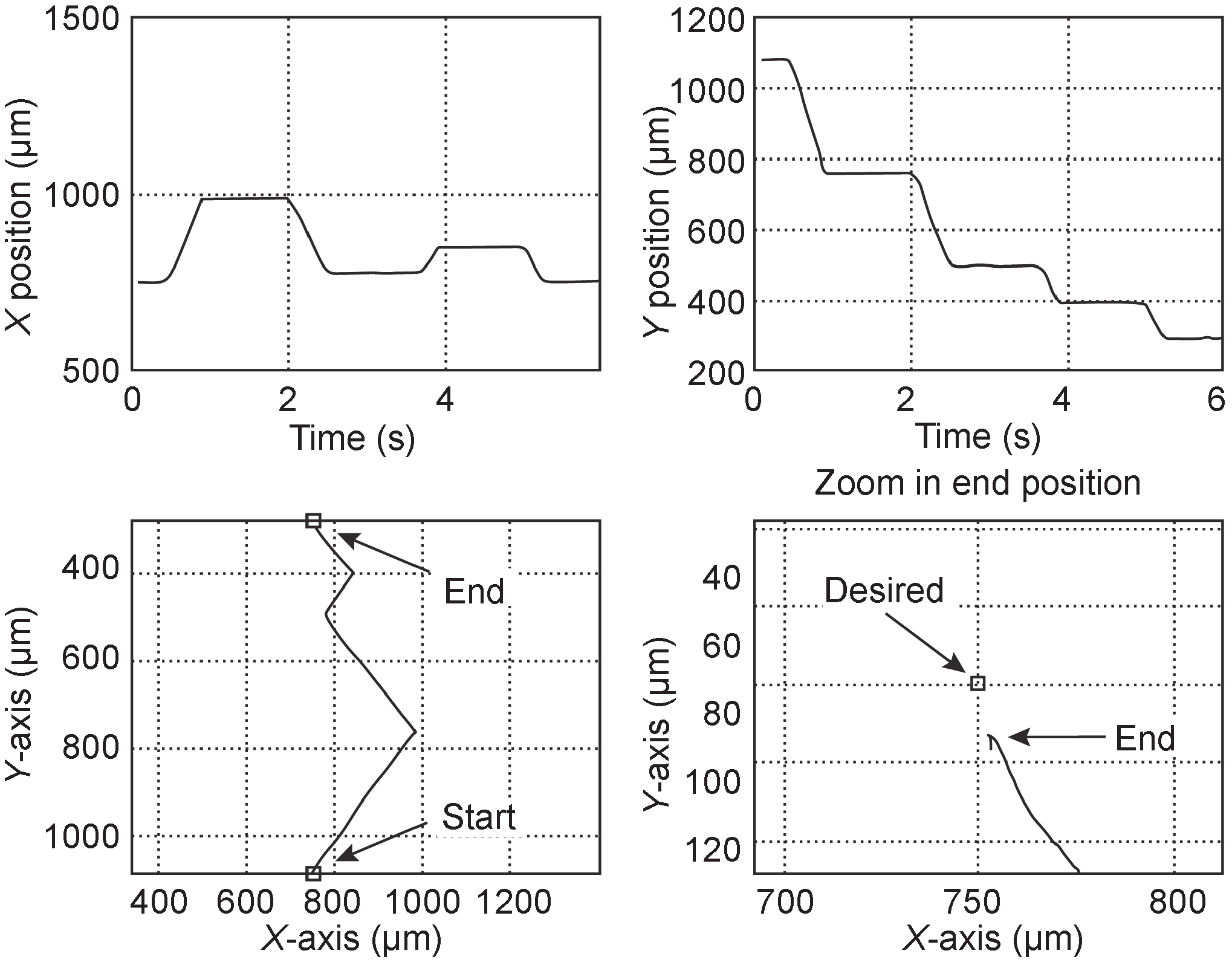
Fig.15 End-effector path and trajectory along the X- and Y-axes using the CL2 methodology of the closed-loop approach.

《Acknowledgements》

Acknowledgements

The authors wish to thank A. Nikolakakis, and C. Dimitropoulos for their assistance in the realization of the experiments.

《Compliance with ethics guidelines》

Compliance with ethics guidelines

Kostas Vlachos, Dimitris Papadimitriou, and Evangelos Papadopoulos declare that they have no conflict of interest or financial conflicts to disclose.