《1. Introduction》

1. Introduction

In the last decade, additive manufacturing (AM)—and laser powderbed fusion in particular—has received significant attention in design and manufacturing processes [1,2]. The technology offers significant design flexibility over the subtractive manufacturing method and has an economic advantage when it comes to customized parts and low volume production. In recent years, the aerospace industry, which is one of  the primary sectors among AM businesses, has started using the AM process to build actual products. GE Aviation, RollsRoyce, Airbus, Boeing, and Pratt and Whitney are among the major companies  that  incorporate  AM  components  into  their  products[3]. Powder is available for use in the AM of several alloys, of which titanium, stainless steel, aluminum, and nickel-based alloys are in common use in today’s market [4]. Inconel 718 is a precipitation hardenable nickel-chromium alloy, which is known for its high yield strength, weldability, and creep-rupture properties, particularly at a high temperature [5]. These properties have made Inconel 718 suitable for the aerospace industry, where severe operating conditions are generally found.

Obtaining the advantages of AM requires control of defects. Common defects in AM parts include lack of fusion because of insufficient energy input (and inappropriate scanning parameters), keyholing from excessive energy input, and the balling effect that results from excessive scanning velocity [6]. These defects can be highly detrimental to the finished part’s mechanical properties, and often induce crack initiation and weak bonding between layers. As the quality of final products strongly depends on the choice of processing parameters, researchers have concentrated on understanding the relationships among part quality, microstructure, mechanical properties, and processing conditions specifically for Inconel 718. Sadowski et al. [7] determined the melt pool shape and size as functions of several processing parameters. This allowed proper operating conditions to be identified that reliably gave fully fused scanning tracks. Wang et al. [5] experimentally studied Inconel 718 parts made by AM and found that microstructures and mechanical properties seemed to be independent of part height. Moreover, columnar microstructures were observed throughout the part, while the quasi-static mechanical properties of AM parts are often comparable or superior to those made by conventional methods.

Even though experimental studies are necessary to characterize AM parts, they are time-consuming and limited to the chosen technique  used.  Mathematical  methods  are  a  supplemental  route to explore and understand the fundamental behavior during the fabrication process. Two major approaches for obtaining results are numerical and analytical solutions. Rosenthal’s analytical model can give a quick estimation (in minutes) of the thermal characteristics of powder-bed fusion [8]. However, the derivation of the Rosenthal equation relies on several simplifying assumptions, which raises concerns about its accuracy and generality. On the other hand, numerical models  often  have fewer  assumptions  than the  analytical solution, which make them more realistic. However, the required calculation time is often drastically longer than that of the former approach. For example, models developed in our research group usually take 4–6 h with an Intel Xeon Processor E5 (2.8 GHz) with four cores to complete a thermal calculation over a 2 mm scanning length (equivalent to approximately 1 ms in physical time)  with mesh numbers around 80 000. Nevertheless, despite these differences, both calculation approaches have been broadly used.

Tang et al. [9] applied the Rosenthal equation along with their proposed criterion to identify conditions that would cause lack of fusion condition in several alloy systems. Their analysis accurately estimates the lack of fusion porosity of as-built parts under various fabricating conditions. In addition, with the analytical solution and existing correlations, Liang et al. [10] developed a process map that can predict the primary dendrite arm spacing (PDAS) in Inconel 718. Results were validated with sets of experiments. Romano et al. [11] used the finite-element (FE) method to calculate melting and solidification in the selective laser melting (SLM) process. Simulation results from Romano et al. tended to overestimate the melt pool width, especially at high power input. Therefore, a correction factor for the effective absorptivity has been proposed to be incorporated with numerical results such that the estimation is in better agreement with measurements. It should be noted that while previous FE studies often consider the powder as a continuum material [2,6,11,12], recent studies by Yan et al. [13,14] have considered the presence of powder particles in the computation domain. Multiscale modeling techniques are introduced to enable comprehensive examination from the powder scale to the layer scale. As a result, Yan’s models represent realistic simulation conditions and can capture complicated physical behaviors such as the interaction between powder particles, as well as the balling effects and the non-uniformity of a scanning track induced by the surface tension. However, such models have high computational cost (reported at 140 h for 4 ms of physical time with an Intel Core i7-2600 processor), and the detailed investigation of defect initiation in a single scanning track is not a primary focus of the present study. Previous studies have shown that both numerical and analytical techniques can be used to describe the AM process and give satisfactory results. However, these two techniques are often studied separately, and a comprehensive comparison between the two approaches is still lacking.

Therefore, the present study aims to comprehensively compare the numerical and analytical solutions in describing Inconel 718 products made by laser powder-bed fusion. Together with existing theoretical criteria, several important parameters of as-built parts including melt pool size, solidification behavior,  and  microstructure will be predicted and compared. The influence of  numerical assumptions on the estimated results of each method will be elaborated. Predictions are confirmed with available experimental data. The analysis spans a wide range of heat input for complete understanding and to ensure the validity of numerical results. The results of this study are expected to strengthen the understanding of the relationship between processing parameters and product outcomes. Moreover, the discussion throughout the paper clearly shows the capability and limitations of the Rosenthal equation to replace or supplement the analysis from the FE model.

《2. Numerical approach: FE modeling》

2. Numerical approach: FE modeling

A three-dimensional (3D) FE model is used to simulate the temperature evolution in the AM process. Temperature-dependent material properties, the Gaussian distribution of the moving heat source, and heat losses from natural convection and radiation are considered. A commercial software, COMSOL, is used to perform the numerical calculation.  Simulation  conditions  in the  present  study replicate typical processing parameters in AM machines, which have a laser power of 150–600 W, a laser spot diameter of 75 µm, a layer thickness of 40 µm, and a scanning velocity of 960 mm•s^–1  [11].

《2.1. Material properties》

2.1. Material properties

The density, specific heat, thermal conductivity, and emissivity as functions of temperature are shown in Fig. 1 [11]. Properties are defined for powder, solid, and liquid phases. In addition, the apparent heat capacity method is used to incorporate the latent heat (L = 210 kJ•kg^–1) due to the phase changing between solid and liquid [15]. The modified specific heat is defined over the melting temperature range ∆T_m, which is about 100 K, centered on an average melting temperature of approximately 1613 K [16] (Eq. (1)).

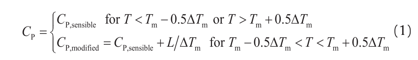
where C_P  and T represent the specific heat and temperature, respectively.

《Fig 1》

 Fig. 1. Thermophysical properties for Inconel 718 as functions of temperature [11]. (a) Density; (b) specific heat; (c) thermal conductivity; (d) emissivity.

《2.2 Thermal model》 

2.2 Thermal model

The thermal model consists of a substrate and powder layer. The substrate and powder layer are 1.5 mm wide and 2.5 mm long. The substrate has a height of 2 mm, and the powder layer has a thickness of 40 µm. In general, the dimension of the substrate that is used in metal AM is larger than the size of the calculation domain. However, the substrate merely acts as a heat sink during the fabrication process; the meaningful thermal participation occurs near the top surface and diminishes rapidly with distance away from the top [11]. It was confirmed with a sensitivity analysis that the calculation domain is sufficiently large to not affect the calculated temperature history and melt pool dimensions, while limiting the computational load. However, it should be noted that at very high energy input, the length of a melt pool could be longer than 2.5 mm. Therefore, if the melt pool length is a major concern, the length of the calculation domain should be appropriately adjusted according to  the  melt pool length. However, to enhance the computational efficiency, and because melt pool depth and width were the primary concerns of the present study, a domain length of 2.5 mm was used. In addition, in the thermal calculation, natural convection in a liquid melt pool is neglected. Neglecting convection would cause the temperature within the melt pool to be overestimated, but would have little effect on the predicted solidification from the edge of the melt pool, where heat transfer is mainly governed by the phase change and heat conduction [17]. The laser power distribution is assumed to be Gaussian, as shown in Eq. (2).
 
       where P is the laser power, r0  is the laser radius, and λ is the absorptivity of the material.

The absorptivity for Inconel 718 has been reported by various researchers; Table 1 [11,18–20] shows that the reported values vary widely, ranging from 0.3 to 0.87. Previous studies summarized in Table 1 used a laser with a wavelength of 1.06 µm, which is comparable to the wavelength of the Yb:YAG laser used in the machine of EOS GmbH, Germany. The experimental study from SainteCatherine et al. [18] indicated that the absorptivity of Inconel 718 tended to increase with higher temperature. To illustrate the sensitivity of the predicted results to the absorptivity, in the present study we performed the numerical analysis for absorptivities of 0.3 and 0.87 as the lower and upper limits, respectively. In addition, the fitted absorptivity that gives the closest estimation of the melt pool width (for the two calculation approaches) will be discussed and shown in Section 4.1.

《Table 1》

Table 1 Reported absorptivity of Inconel 718 for a laser wavelength of 1.06 µm.

Radiation from the top surface is quantified using a heat transfer coefficient for radiation:

where  h_rad  is the heat transfer coefficient for radiation, σ is the StefanBoltzmann constant, ε is the emissivity, and T_∞ is the ambient temperature. 

The boundary condition at the bottom of the substrate is main-tained at room temperature, based on the experimental observation that the measured temperature at the substrate shows insignificant change during the process [6]. The side walls are assumed to be insulated. Fig. 2(a) summarizes the thermal boundary conditions used for numerical modeling in the present study, while Fig. 2(b) illustrates the bulk 3D geometry considered in the FE calculation.

《Fig 2》

Fig. 2. (a) Thermal boundary conditions: ① laser heat input on the top surface; ② heat losses due to convection and radiation; ③ insulated walls; ④ constant temperature at the bottom. (b) Bulk 3D geometry considered in the FE calculation.

《3. Analytical approach: Rosenthal equation》

3. Analytical approach: Rosenthal equation

Rosenthal [8] originally developed the analytical method to predict the temperature history in fusion welding. Because of similarities between fusion welding and SLM, the Rosenthal equation is extended to predict the thermal characteristic in laser melting. The Rosenthal equation owes its merit to its simplicity and wide applicability. Moreover, this single formula is capable of predicting temperature history as a function of time, temperature gradient, cooling rate, and solidification rate. The Rosenthal equation was derived based on the following assumptions:
•    The thermophysical properties, including thermal conductivity,density, and specific heat, are temperature independent. The latent heat due to phase change is not included.
•    The scanning speed and power input are constant, leading to a  quasi-stationary  condition  of  the  temperature  distribution around the melt pool.
•    The heat source is a point source.
•    Heat losses from surface convection and radiation are not considered, and convection in the liquid pool is neglected. Therefore, the heat transfer is governed purely by conduction.
 
     To use the Rosenthal equation in a powder-bed process, an additional assumption is made: that the deposition of powder has an insignificant influence on melt pool size. Montgomery et al. [19] and Gong et al. [21] confirmed the validity of this assumption through their experiments under processing conditions similar to those used in the present study. Single scanning tracks were made on a solid substrate with and without the presence of powder; the melt pool areas were similar, and the melt pool widths in the no-powder cases were only slightly larger than those with powder. This showed that the difference in melt pool width is insignificant in the context of this work.

The resulting analytical solution, that is, the Rosenthal equation, is as follows:
 

where T₀  is the temperature at locations far from the top surface, k is the thermal conductivity, V is the scanning velocity, and α is the thermal diffusivity. It should be noted that in Eq. (4), the laser moves along the x-axis, in which the moving coordinate of x − Vt is replaced by ξ; r is the distance from the heat source, defined as (ξ² + y² + z²)^0.5. Since the Rosenthal equation does not account for any temperature-dependent material properties, the properties at room temperature, as shown in Table 2 [11], were used.

《Table 2》

Table 2 Room-temperature thermal properties of Inconel 718 used in the Rosenthal equation.

《4. Results》

4. Results

A comparison between the  Rosenthal equation, the FE  model, and the experimental results is performed for various values of heat input. The heat input calculated from the laser power and scanning velocity is shown in Eq. (5). Both parameters are important because they affect the melt pool configuration and the thermal behavior in a scan track.

Fig. 3 shows the temperature contour and melt pool boundary, as obtained from the FE model. Thermal results from the FE calculation enable further calculation of the melt pool dimensions, solidification rate, and temperature gradient, and thus allow a prediction of the solidification  microstructure.  The  following sections  compare the results of the numerical and analytical calculations with measured results from the experiment. The temperature gradient and solidification rate obtained from two approaches will be reviewed, as these parameters are important in microstructure prediction. Furthermore, the solidification map and the PDAS obtained from two approaches will be discussed.

Fig. 3 shows the temperature contour and melt pool boundary, as obtained from the FE model. Thermal results from the FE calculation enable further calculation of the melt pool dimensions, solidifica-tion rate, and temperature gradient, and thus allow a prediction of the solidification microstructure. The following sections compare the results of the numerical and analytical  calculations with meas-ured results from the experiment. The temperature gradient and solidification rate obtained from two approaches will be reviewed,as these parameters are important in microstructure prediction. Fur-thermore, the solidification map and the PDAS obtained from two approaches will be discussed.

《Fig 3》

Fig. 3. (a) Cross-sectional view (y–z) of the temperature contour (°C) and melt pool boundary (indicated by the black line) from the FE model; (b) longitudinal view (x–z) of the temperature contour (°C) and melt pool boundary (indicated by the black line) from the FE model. Simulated with a laser power of 200 W, scanning velocity of 960 mm•s^–1, and absorptivity of 0.5.

《4.1. Melt pool configuration from experimental, numerical, and analytical results》

4.1. Melt pool configuration from experimental, numerical, and analytical results

An example of a plot of the melt pool boundary (based on the Rosenthal equation) is shown in Fig. 4. The melt pool width is at its maximum when dy/dξ = 0; Tang et al. [9] showed that the following expression (derived from the Rosenthal equation) can be used to estimate the melt pool width for materials (such as Inconel 718) with relatively low thermal diffusivities:

where ρ is the density and W is the melt pool width.

《Fig 4》

Fig. 4. Plan view of a Rosenthal plot of the melt pool boundary, calculated for Inconel 718 with an absorbed power of 142 W and with V = 960 mm•s–1. The point heat source is at the intersection between the horizontal and vertical axes. W is the melt pool width and D is the melt pool depth.

It  should  be  noted  that  the  conditions  behind  the  Rosenthal equation lead to a predicted semi-circular melt pool cross-section (perpendicular to the beam travel direction). Thus, the calculated melt pool depth is half of the melt pool width.

Experimental results were compared with the predicted melt pool widths: Sadowski et al. [7] experimentally investigated the effect of processing parameters on the quality of additively manufactured parts. Samples were made in an EOSINT M 280 (EOS GmbH, Germany) with Inconel 718 powder. Experimental parameter variations included beam power ranging from 40 W to 300 W, scanning velocities from 200 mm•s^–1 to 2500 mm•s^–1, a hatch spacing of 110 µm, and a laser spot diameter of 75 µm. The processing parameters in the experimental study are consistent with those used in the numerical simulation, as mentioned in Section 2. Since these experiments covered a broad range of laser powers and scanning velocities, they are used for validation and comparison against the predictive capability of the numerical and analytical calculations.

Fig. 5 compares the average experimentally measured line widths (which are taken to be the same as the melt pool widths) with predictions from the Rosenthal equation and the FE model. The average line width is measured on single beads imaged in plan views of the specimen [7]. Numerical estimations are performed by varying the absorptivity from 0.3 to 0.87 in order to illustrate the sensitivity of the prediction. The fitted absorptivities that yield the closest agreement with the experiment are found to be 0.4 for the Rosenthal equation and 0.5 for the FE model. Based on fitting results, it is seen that the predictions and measured results are in good agreement up to a heat input of 0.4 J•mm^–1. At higher heat inputs, the FE approach tends to slightly underestimate the melt pool width, while the Rosenthal equation overestimates the width. Micrographs indicate that keyholing occurs at high heat inputs [7]; keyholing leads to narrower and deeper melt pools. The smaller melt pools predicted by the FE approach could be affected by excessive radiative losses from the surface; because melt pool convection is not included in the FE calculations, the predicted melt pool surface temperature is too high, resulting in an overestimate of radiative losses. In contrast, the Rosenthal approach completely neglects radiative losses from the melt pool surface.

《Fig 5》

Fig. 5. Melt pool width comparison between the experimental results from Ref. [7] and predictions from the Rosenthal equation and the FE model. The shaded area shows the range  of  predictions  when  varying  the  absorptivity  from  0.3  to  0.87,  while the  dashed  lines  show  the  fitted  absorptivity  of  the  two  approaches.

Regarding the sensitivity of predictions to absorptivity, Fig. 5 shows that the Rosenthal equation is more sensitive to absorptivity, especially at very high heat input, compared with  the FE model; this result further confirms the significant influence of radiative and convective heat losses from the surface, as these are incorporated in the FE model but not in the Rosenthal equation.

《4.2. Thermal predictions: Temperature gradient, cooling rate, and solidification  rate》

4.2. Thermal predictions: Temperature gradient, cooling rate, and solidification  rate

The solidified microstructure is governed by thermal conditions such as temperature gradient (G) and solidification rate (R) during solidification. The Rosenthal equation enables a quick estimation of these parameters through derivation from Eq. (4). The following equations give the temperature gradient in the ξand z-directions. Eqs. (7) and (8) were derived for the melt pool cross-section in the ξ-z plane at y = 0 (refer to the coordinates in Fig. 3(b)). The local cooling rate (∂T/∂t) can be found from Eq. (9).
  

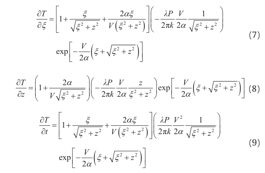
The temperature gradient, cooling rate, and solidification rate vary significantly at different locations within the melt pool, as shown in a previous study by Bontha et al. [22]. The partial remelting of previously deposited layers is required during the AM process in order to fuse the new layer to the layer below it, and to avoid the gaps that result in a lack of fusion voids. However, the present study uses the average thermal behavior from the bottom of the melt pool, which is formed during the deposition of layer n, up to the bottom of the melt pool of the next layer, n + 1 (Fig. 6). In other words, the thermal behaviors are averaged over a region that does not experience remelting from the next deposited layer. The rationale is that the final as-deposited microstructure depends only on the thermal history in the last melting step, and that the previous melting steps are not significant to microstructure formation. Therefore, the thermal behaviors obtained as shown in this section are used for the microstructure prediction in subsequent sections.

《Fig 6》

Fig. 6. Illustration of the melt pools in two layers; regions with and without remelting are identified.

Determining  the  temperature  gradient  and  cooling  rate  starts with finding the melt pool depth from Eq. (6). Next, Eq. (4) is solved in order to determine the ξ and z coordinates along the melt pool boundary from the bottom of the melt pool up to a position 40 µm above the bottom of the melt pool (where 40 µm is the layer thickness in the present study). The set of ξ and z values at various locations is used to determine the local thermal behavior from Eq. (7) to Eq. (9), and the average values are obtained to be compared with results from the FE model. The solidification rate is determined from the total temperature gradient and cooling rate, as displayed in Eq. (10). The analytical solution is computed using the MATLAB software package.
 

Similar to the Rosenthal equation, in order to obtain the thermal behavior from the FE model, the melt pool depth is first determined. Next, the temperature history and temperature gradient of various locations along the melt pool, which do not experience remelting, are obtained, as described earlier in this section. For better understanding, the example case that uses 200 W laser power, 960 mm•s–1 scanning velocity, and an absorptivity of 0.5 is shown. Under these processing conditions, the estimated melt pool depth is 69 µm. The thermal histories  are  evaluated  at  five  different  locations:  5 µm, 10 µm, 20 µm, 30 µm, and 40 µm above the bottom of the melt pool. Fig. 7(a) and Fig. 7(b) show the temperature and temperature gradient in the z-direction as a function of time, while Fig. 7(c) displays the temperature gradient as a function of temperature during the cooling process. The temperature gradient at the melting temperature is extracted, while the average value is calculated and compared with the results from the Rosenthal equation. The average cooling rate is also extracted using the same approach as the temperature gradient, and the temperature gradient and cooling rate are used to calculate the solidification rate using Eq. (10).

 《Fig 7》

 Fig. 7. (a) Temperature as a function of time from various locations within the melt pool; (b) temperature gradient as a function of time from various locations within the melt pool; (c) temperature gradient as a function of temperature from various locations within the melt pool during the cooling process. Simulated by the FE model with a laser power of 200 W, scanning velocity of 960 mm•s^–1, and absorptivity of 0.5.

The thermal behavior comparison between the Rosenthal equation and the FE model is shown in Fig. 8. The analysis is performed for various heat inputs, where the scanning velocity is fixed and the laser power is altered to achieve a desired energy input. Fig. 8(a)– Fig. 8(c) show that both approaches predict the same trend in the temperature gradient, which becomes smaller at a higher heat input. The major contribution comes from the larger melt pool size and larger high-temperature region that are associated with a higher energy input, which eventually attenuates the temperature gradient within the melted region. Based on the fitted absorptivity, the temperature gradients from the Rosenthal equation and the FE model are very similar, whereas the cooling rate and solidification rate from the FE model are slightly higher than those from the Rosenthal equation.

《Fig 8》

Fig. 8. A comparison of (a) temperature gradient, (b) cooling rate, and (c) solidification rate from the Rosenthal equation and the FE model. The shaded area indicates sensitivity to absorptivity in the range 0.3–0.87. Dashed lines indicate results from the fitted absorptivities of 0.4 and 0.5 for the Rosenthal equation and the FE model, respectively.

In addition, as  seen from the  melt pool  configuration prediction, the discrepancy in the predictions of the cooling rates from the Rosenthal equation and the FE model is small at a low energy density and becomes larger with a high energy input. One of the explanations could be the difference in predicted melt pool size, for which the contribution from radiative and convection losses could play an important role at a high energy density. By neglecting heat losses, the Rosenthal equation would have a higher overall heat input than the FE model, which could eventually lead to a lower cooling rate. Furthermore, since the temperature-dependent thermal conductivity at the melting temperature is three times higher than at room temperature, the higher thermal conductivity accelerates the cooling during the solidification in the FE simulation. The difference in the cooling rate predictions from the two approaches varies from 10% to 60%. A comparison between the Rosenthal equation and the FE model was previously carried out by Goldak et al. [23] for the cooling rate prediction in the welding. Compared with experimental results, they reported that the FE model underestimates the cooling rate by 5%, while the Rosenthal equation shows an overestimation of 41%. Their results differ from the results of the present study, which show that the cooling rate from the FE model is higher than that from the Rosenthal equation. A possible explanation could be that the material used in the study by Goldak et al. [23] was low-carbon steel, for which the thermal conductivity is reported to be lower at higher temperatures, possibly resulting in a lower cooling rate when temperature-dependent thermal conductivity is considered. In addition, the cooling rate prediction from both approaches is highly sensitive to the choices of absorptivity at low energy density, as seen from the sensitivity study. However, the effect of absorptivity on cooling diminishes at a higher heat input, when the cooling rates are inherently lower.

Note that the thermal analysis is performed under the assumption that the initial temperature is close to room temperature. However, this assumption will not hold when significant accumulation of heat occurs. Factors that promote local temperature rise include a short resting time between layers, which leads to less cooling time; an extremely small scanning length, which creates a rapid temperature rise in layers; or geometry containing very small features, which results in poor heat conduction due to the low thermal conductivity of the surrounding powders. If any of these factors occur, the Rosenthal equation will be inapplicable unless the initial temperature can be independently computed; in contrast, a full FE analysis can account for specific geometries.

《4.3. Microstructural predictions: Solidification map and PDAS》

4.3. Microstructural predictions: Solidification map and PDAS

The ability to predict the solidification  microstructure  will lead to a better understanding of the interplay between the processing parameters and the microstructure. This knowledge will contribute to the prediction of mechanical properties in additively made products. Fig. 9 shows a solidification microstructure map. This kind of map is particularly useful for illustrating the as-built microstructure after solidification, where the microstructure is controlled by the temperature gradient and solidification rate [24].There  are  three  possible  solidified  microstructures:  columnar, mixed, and equiaxed. The results from the Rosenthal equation and the FE model are plotted separately in maps that contain results for various heat inputs and various locations along the melt pool, as shown in Fig. 9. Note that only results from fitted absorptivity are shown. Energy densities vary from 0.16 J•mm^–1   to 0.63 J•mm^–1, and the plotted locations are 5 µm, 10 µm, 20 µm, 30 µm, 40 µm, and 50 µm above the bottom of the melt pool. Fig. 9 shows that the plots of the solidification maps from the Rosenthal equation and the FE model are mostly indistinguishable in the log scale, in which both approaches predict a columnar microstructure. This observation agrees well with a study by Wang et al. [25], which reported that a fine columnar dendritic structure, which grows epitaxially along the [001] crystallographic orientation from the bottom of  the melt pool, is generally found in AM parts made by Inconel 718. However, the agreement of the solidification maps with the observed microstructures might be fortuitous: The boundaries of the columnar and equiaxed microstructures were calculated for conventional castings [26]; however, in laser powder-bed fusion, the small melt pool, dominant role of epitaxial grain growth from the melt pool boundary, and  high  solidification  rate  would  all  affect the applicability of the solidification map.

《Fig 9》

Fig. 9. A comparison of the solidification maps from (a) the Rosenthal equation and (b) the FE model. Results are from an absorptivity of 0.4 (Rosenthal equation) and 0.5 (FE model).

In addition to grain types, PDAS is an important microstructure feature that affects the mechanical properties [10]. Therefore, various researchers have studied the connection between solidification behavior and the PDAS [27,28]. One of the most common models is the Kurz and Fisher (KF) model [28]. The KF model (Eq. (11)) has been proven to be effective and reasonably accurate in determining the PDAS in nickel-based superalloy products [29].

where δ is the PDAS (µm), G is the thermal gradient (K•m^–1), and R is the solidification rate (m•s^–1). ∆T0 , D, k0 , and Γ are material properties, and are summarized in Table 3 [10,16].

《Table 3》

Table 3
 
 

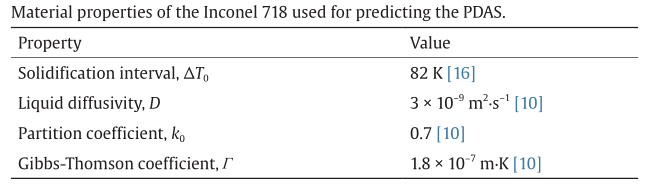
Fig. 10 shows the PDAS predictions from analytical and numerical approaches for various heat inputs. Both calculation approaches predict the expected trend of PDAS increasing with higher heat input, as was experimentally observed by Wang et al. [25]. The PDAS prediction from the Rosenthal equation is slightly larger than that from the FE model: The difference between these two methods is up to 29%. To validate the numerical results, experimental data obtained under similar processing conditions to the numerical calculations is used for comparison. Lee and Zhang [20] experimentally performed the PDAS measurement from Inconel 718 parts made in an EOSINT M 280 (EOS GmbH, Germany). The reported PDAS values from their study are 1–1.8 µm at an energy density of 0.3 J•mm^–1. The predictions from both the Rosenthal equation and the FE model are in good agreement with the experimental data. However, even though both methods show that they can reasonably predict the PDAS, insufficient experimental data makes  it  difficult  to  identify the better model in predicting the PDAS. Thus, more experimental data, especially at different energy densities, is essential in order to provide better confidence in analytical and numerical predictions; more data will also allow the identification of better approaches.

《Fig 10》

Fig. 10. A comparison of PDAS predictions from the Rosenthal  equation  and  the  FE model, and the experimental result from Ref. [20].  The  shaded  area  indicates  the  result’s sensitivity for various absorptivities from 0.3 to 0.87. Dashed lines indicate the results from the fitted absorptivities of 0.4 and 0.5 for the Rosenthal equation and the FE  model,  respectively.

《5. Conclusions》

5. Conclusions

The present study examines the thermal behavior in parts made from Inconel 718 by SLM. The investigation uses both an analytical solution (the Rosenthal equation) and the FE method. The analysis includes determination of the melt pool configuration, solidification behavior, grain type prediction, and PDAS. The predicted results are compared with experimental results from the literature. The two approaches are also compared in order to examine the similarities and differences in their predictive capability. The conclusions are as follows:
(1)    Both the Rosenthal equation and the FE model predict the melt pool dimensions with good agreement at an energy density less than 0.4 J•mm^–1. However, at a higher energy density, the predicted melt pool size from the Rosenthal equation is greater than that from the FE model; this could be a consequence of assumptions such as neglecting latent heat and heat losses at the surface.
(2)    Based on fitted absorptivity values, the temperature gradient estimations from both approaches are in good agreement, whereas the cooling rate and solidification rate from the FE model are higher than those from the Rosenthal equation.
(3)    Since the Rosenthal equation does not account for heat losses, its prediction of the melt pool size and the cooling rate is more sensitive to choices of absorptivity than that of the FE model.
(4)    Based on a solidification map, both approaches predict columnar growth, which agrees with experimental results. Moreover, due to the log scale plot, the results from the Rosenthal equation and the FE model are indistinguishable on the solidification map.
(5)    The PDAS prediction from the Rosenthal equation is larger than that from the FE model, with a maximum difference of up to 29%. However, compared with an experimental result at the energy density of 0.3 J•mm^–1, both methods can reasonably predict PDAS. Nevertheless, more experimental PDAS data will be required to differentiate which model is better, especially as a function of energy density.
(6)    Ultimately, the Rosenthal equation and the FE model provide similar and reasonable thermal and microstructural results at a low energy input, with the Rosenthal equation being useful for quick estimation. However, at a high energy input, the Rosenthal equation should be used with caution because heat losses, which are neglected, can become dominant. Therefore, the FE model is more accurate at a high energy input because it incorporates more realistic material properties.

《Acknowledgements》

Acknowledgements

Patcharapit Promoppatum is grateful for support from the Royal Thai Government and the Bertucci Graduate Fellowship for this research. P. Chris Pistorius and Anthony D. Rollett acknowledge support from Early Stage Innovations under National Aeronautics and Space Administration (NASA)’s Space Technology Research Grants Program (NNX 17AD03G).

《Compliance with ethics guidelines》

Compliance with ethics guidelines

Patcharapit Promoppatum, Shi-Chune Yao, P. Chris Pistorius, and Anthony D. Rollett declare that they have no conflict of interest or financial conflicts to disclose.