《1. Introduction》

1. Introduction

Traditional energy generation uses fossil-fuel resources such as oil, natural gas, and coal, which are depleted with consumption [1] and cause environmental pollution and global warming. For example, the use and combustion of fossil fuels cause toxic air emissions that result in environmental problems with great risk to living organisms [2]. Carbon dioxide (CO₂) accounts for an estimated 77% of human-generated greenhouse gas emissions [3]. These factors contribute to toxic air emissions in the environment by harming the climate. Therefore, it is currently of the utmost importance to exploit new ways of producing energy that is more environmentally friendly, economical, clean, and inexhaustible by nature. Renewable energy sources (RESs) are an emerging trend and are widely used to generate power from various sources, including solar, wind, geothermal, hydropower, and other naturally replenishing energy sources [4]. Among RESs, wind turbines (WTs) and photovoltaics (PVs) are the most dominant and encouraging technologies, and are considered by the global community to fulfill the load requirements of electricity consumers [5].

RESs that consist of solar and wind systems have come under more focus than other energy sources because they tend to reduce ecological and universal CO₂ emissions [6,7]. However, such resources can be unpredictable and intermittent, depending on natural conditions. The reliability of RESs is thus a major concern that needs to be tackled at a minimum cost to consumers. To overcome environmental challenges, there is a great need to consider RESs in energy production. RESs can be implemented in two ways: grid-connected (GC) and stand-alone (SA) modes. In GC modes, RESs inject the produced electricity to a power utility network, while in SA modes, they directly power up the consumer’s electrical load [8].

In a GC system, the consumers are directly connected to the utility grid. In case of any shortfall of electricity from the RESs, consumers can obtain and fulfill their load requirements from the utility grid. Thus, there are no reliability concerns in the GC system. An SA system introduces unreliability concerns because consumers are only dependent on the power produced by the RESs, and there is no connectivity to a grid system. Furthermore, using a single RES in an SA environment results in high energy variations. This effect results in an energy mismatch situation, where the consumer’s load requirements are not fulfilled by the generation capacity. To overcome RES unreliability and related challenges, Ref. [9] utilizes a hybrid renewable energy system (HRES) along with an energy storage system (ESS) to fulfill the consumer’s load. The complementary features of solar and wind energies are combined in the HRES, along with ESS backup. An ESS, which consists of batteries, fuel cells (FCs), and other technologies, is utilized to satisfy the deficit energy during stress time—that is, when the energy produced by RESs is less than the required load. Therefore, the power solution provided by an HRES along with an ESS is considered to be more sustainable and reliable than a single RES [10].

The primary issue in an HRES is determining the optimum size of individual components, including WTs, PVs, and batteries. Optimal sizing is required for strategic decisions such as feasibility studies, initial capital investments, or cost estimations. The methodology used to determine accurate and appropriate sizing of HRES components by maintaining the system’s reliability at minimal total annual cost (TAC) is called unit sizing [11]. The unreliability of RESs can be overcome by oversizing the system’s components; however, doing so results in an increased system cost. On the other hand, undersizing the system’s components can lead to a loss of supply (LOS) problem, in which the energy produced by the RESs is less than the consumer’s load. Therefore, optimum unit sizing of an HRES that measures the exact number of a system’s components at a reduced TAC is essential [12]. (Nomenclature is provided at the end of this paper.)

Software-based tools, formal techniques, and meta-heuristic algorithms are commonly used for the unit sizing of RESs. The hybrid optimization model for electric renewables (HOMER) is a software-based tool that is applied for energy optimization, sensitivity analysis, and planning. Mamaghani et al. [13] suggest the use of a PV–WT–diesel generator HRES for electrifying three remote off-grid villages in Colombia. A techno-economic feasibility analysis of the cost and an environmental evaluation in terms of CO₂ is conducted. The HOMER software tool is used for the technoeconomical HRES analysis in order to fulfill 13 048 kW of average load requirements per day, with an estimated peak of 1185 kW [14]. The PV–WT–diesel–battery system provides optimal results of 17.15 million USD and 2 571 131 kg per year in terms of net present cost (NPC) and CO₂ emissions, respectively. In contrast, the electricity produced by a single diesel generator results in an NPC of 21.09 million USD and 5 432 244 kg per year of CO₂ emissions. Karmaker et al. [15] conduct an environmental and economic feasibility assessment of the use of a PV–biomass–battery system to supply power to electric vehicles in Bangladesh. Results are obtained by means of the HOMER Pro software, which shows a 34.68% deduction in CO₂ emissions with the use of the proposed system in contrast to grid-based electric vehicle charging, along with savings of 12–18 USD per month. The HOMER software used in Refs. [13–15] suffers from some limitations and is not capable of performing multi-objective optimization; it only supports a uniobjective function based on NPC minimization. In addition, HOMER does not support intra-hour basis variability, and requires a huge computational time for large design points.

Considering the limitations of the HOMER software, works like Refs. [16–18] solve the optimal unit sizing of RESs through mixedinteger linear programming (MILP). Ren et al. [16] consider a GC scenario in which residential energy demands are fulfilled through a PV–FC–battery system. The authors propose a multi-objective function to reduce both annual cost and CO₂ emissions. The authors formulate the problem via MILP and consider selling energy back to the grid. The results demonstrate that batteries contribute to economic benefit while PVs provide an environmentally friendly solution. However, the MILP is a formal technique that suffers from some limitations. The MILP technique performs a complete search of the solution space to find an exact solution. However, this technique is not suitable for stochastic environments and suffers from the curse of the dimensionality problem for large design points.

Other studies have suggested the use of meta-heuristic algorithms, including the artificial bee swarm optimization (ABSO) [19], genetic algorithm (GA) [20–22], harmony search (HS) [23,24], and particle swarm optimization (PSO) [25–27], among others, which are more successive and highly efficient [28] in comparison with other approaches. However, techniques such as the HS, PSO, GA, and ABSO require algorithmic-specific parameters in order to function. For example, the HS algorithm uses harmony memory, pitch adjustment, and the consideration rate with several improvisations, while the PSO requires cognitive and social parameters with inertia weight values. The GA needs a selection operator along with crossover and mutation probabilities. Similarly, the ABSO cannot be executed without initialization and adjustment of algorithmic-specific parameters including the number of employed, scout, and onlooker “bees” with a limit specifier. Algorithms such as GA and ant colony optimization also require performance tuning of algorithmic-specific parameters in order to achieve optimal results. If not tuned properly, algorithmicspecific parameters may result in locally optimal solutions or an increased computational time.

Meta-heuristic algorithms such as PSO, ABSO, and GA require not only algorithmic-specific parameters, but also performance tuning of their parameters in order to achieve an optimal solution. The performance of these algorithms is mainly dependent on the selection, calibration, and performance tuning of these parameters. A small change in any parameter may affect the overall performance of the algorithm and may result in increased computation time or being stuck in local optima. Therefore, algorithms have been proposed in the literature, including Jaya [29], teaching– learning-based optimization (TLBO) [30], and improved TLBO [31], which do not need any algorithmic-specific parameters. Furthermore, the functioning of these algorithms is only dependent on certain common controlling parameters such as number of generations and population size.

This paper solves the unit sizing problem of an HRES via the Jaya, TLBO, and their hybrid, JLBO, algorithms. We consider a hybrid PV–WT–battery system, which is more ecofriendly and cost-effective than other hybrid systems utilizing diesel generators. The contributions listed below are an extension of our previous work [32]:

• Various components of the PV–WT–battery system are formulated and elaborated using an informative HRES model.

• Motivated by non-algorithmic-specific approaches, Jaya and TLBO algorithms are proposed to find an optimal number of HRES and their components to reduce the user’s annual electricity cost in an SA environment.

• A hybrid approach, JLBO, is proposed by combining Jaya and the learning phase of the TLBO algorithm for optimized searching of the solution space.

• The reliability of the system is considered using the various maximum allowable loss of power supply probability (LPSP_max) values provided by the consumer.

The rest of the paper is organized as follows. Section 2 depicts the proposed system model, sizing formulation, and objective function based on some constraints. The methods are given in Section 3. Simulation results are presented and discussed in Section 4. A conclusion and future work are provided in Section 5.

《2. System model and sizing formulation》

2. System model and sizing formulation

This section comprises the system model and the formulation of RES and TAC modeling.

《2.1. The proposed system model》

2.1. The proposed system model

Fig. 1 displays a typical system model for a PV–WT–battery HRES. The proposed system model consists of a single direct current (DC) bus architecture. The bus is connected to dual RESs, including PV panels and WTs. The intermittent nature of solar and wind systems can cause nonlinear and unpredictable output power from RESs. Thus, using a single RES in an SA mode would result in energy variations. Therefore, an HRES comprising solar and wind systems is used in conjunction with an ESS. The ESS is composed of batteries, which are kept in a battery bank. Conventionally, the ESS uses deep-cycle lead-acid batteries.

《Fig. 1》

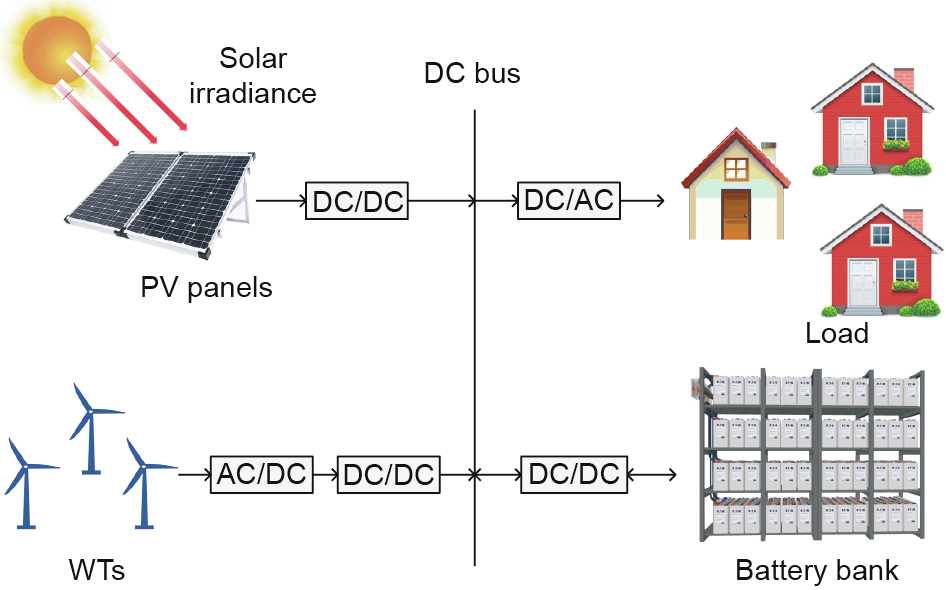
Fig. 1. Proposed system model for an HRES. AC: alternating current; DC: direct current.

Three different modes—balance, surplus, and deficit—are defined for the power generation from the RESs. In balance mode, the total power generated from RESs, including WTs and PVs, is equal to the total consumer’s load. Thus, there are no surplus or deficit powers. In surplus mode, the total energy produced by the RESs is greater than the total consumer’s load; therefore, the ESS is utilized and the additional energy is stored in the batteries of the power bank. Here, the flow of power is from the RESs to both home and ESS. In the power deficit mode, the RESs produce less power than is required by the user. Thus, the ESS is utilized to fulfill the consumer’s load in power deficit time slots. Here, the flow of power is from both the RESs and the ESS to the consumer’s load. Thus, the ESS in conjunction with RESs adds a reliability factor and makes the hybrid model economical for the user.

《2.2. Sizing formulation of the proposed model》

2.2. Sizing formulation of the proposed model

This section presents the modeling of the RESs, ESS, and TAC.

(1) Sizing formulation of the PV power system. The hourly PV panel power output POW^pv for solar radiation I is given by Eq. (1) [19]:

where POW^pv(t ) is the total hourly PV panels’ power (W) generated at time slot t,  is the rated PV power, I represents the solar insulation data (W∙m^-2 ), I ^ref denotes the solar insulation under the reference conditions with a value of 1000 W∙m^-2 , and T ^cof is the temperature coefficient of the PV panels and is set as –3.7 × 10^-3 °C^-1 for mono- and polycrystalline silicon [19]. T ^ref represents the PV cell temperature under the given reference conditions, which is normally set as 25 °C, while T ^c represents the cell temperature, which can be obtained by Eq. (2):

where T ^amb depicts the ambient air temperature (°C), and T noct represents the normal operating cell temperature (°C). T noct is dependent upon the manufacturer’s specifications for the PV module.

If there exist a number of PV panels N ^pv , then the total generated power can be given as follows:

(2) Sizing formulation of the WT power system. The mechanism of the WT generator that produces electrical power is entirely based upon the wind’s kinetic energy. The WT may be composed of two or more blades that are mechanically coupled to a motor that generates power depending on the speed of the wind. To increase the WT efficiency, the turbine is mounted high on a tower. The WT power POW^wt at time slot t is calculated by the following equation [33]:

where represents the speed of the wind;  denotes the nominal power of WT; and represent the rated, cut-out, and cut-in wind speed, respectively. The parameters x and y can be obtained by Eq. (5):

If there are the number N ^wt of WTs installed in an area, then the overall produced wind power is obtained by the following equation:

(3) Accumulative power generation by RESs and the consumer’s load formulation. The PV and WT accumulative electricity generation can be expressed as follows:

where represents the efficiency of the inverter.

In homes, the consumer’s load at time slot t depends upon the appliances’ usage. Thus, the can be computed by Eq. (8):

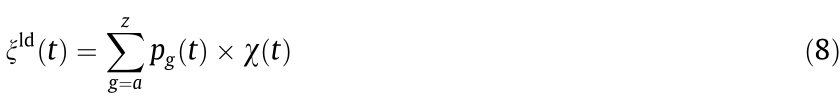
where g and p denote the number of appliances and their power ratings, respectively. represents a Boolean integer showing an appliance status. When = 1, the appliance status is considered to be ON at hour t ; otherwise, it is considered to be OFF.

(4) Sizing formulation of the battery bank. The energy storage capacity of the battery bank is changed due to the intermittent nature of solar irradiation and wind speed. When is greater than , the battery bank is in a state of charge (SOC). Thus, the charging quantity of the battery bank at time slot t is obtained  by Eq. (9) [19]:

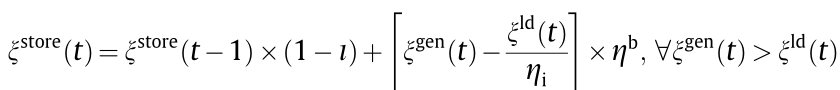
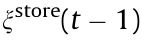where and show the stored amount of energy in the battery bank at time slots t and (t – 1), respectively; represents the self-discharging state; and denotes the battery bank charging efficiency.

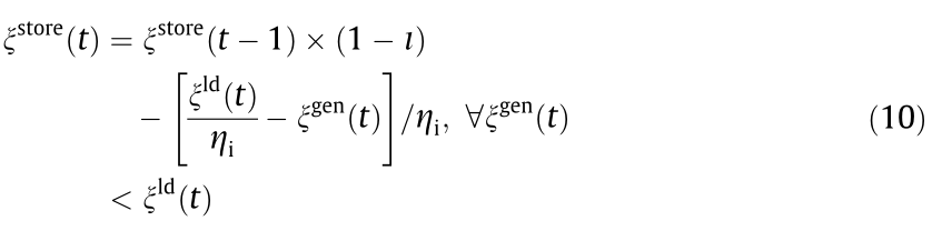
When is less than at time slot t , the stored energy in the battery bank is utilized to fulfill the consumer’s load. Here, the state of the battery bank is changed to discharging. The battery bank discharging efficiency is assumed to be 1, and temperature effects are not considered for this study. Thus, the battery bank charging quantity at time slot t is given by the following formula:

《2.3. Calculation of batteries for the battery bank》

2.3. Calculation of batteries for the battery bank

An important decision variable in the PV–WT–battery HRES is the calculation of the total number of batteries (N ^b ) required for the battery bank. N ^b depends upon the consumer’s load requirement and the generation capacity of the RESs. To find N ^b , a temporary storage variable (temp) is supposed and initialized as 0. When the power generation from the RESs is higher than the consumer’s load at an instant of time slot t, the temp stores energy, as per Eq. (9). However, when the power generation produced by the RESs is smaller than the consumer’s load at time slot t, the temp variable is updated using Eq. (10). Thus, finding the total number of batteries for a system is dependent upon the curve of the variable temp. Positive temp values indicate the generation availability of the RESs, while negative values show a generation deficiency in the respective time slots. The total required storage capacity (T ^rsc ) is the difference between the maximum point and the minimum point in the temp curve, which can be obtained by the following equation:

where, max(temp) and min(temp) represent the maximum and minimum generation points on the temp curve, respectively. Thus, the calculation for the N ^b required for a given system can be derived using the following equation [34]:

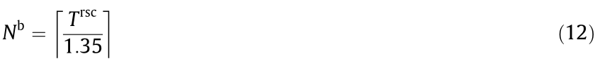
where 1.35 is the nominal capacity of a battery.

《2.4. System reliability》

2.4. System reliability

Reliability is an essential factor that must be considered in the SA system. Therefore, in this paper, the concept of the loss of power supply probability (LPSP) is considered and implemented to obtain a reliable HRES. The LPSP is elucidated by a number in the range of 0 and 1. An LPSP of 0 indicates that the system is very reliable and the consumer’s load will always be fulfilled. An LPSP equal to 1 indicates that the consumer’s load is never fulfilled. The LPSP for one year (T = 8760 h) can be expressed as follows:

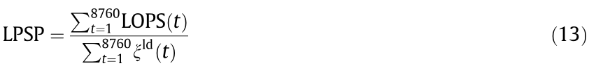
where LOPS stands for loss of power supply. LOPS occurs when the total energy generated by the HRES is less than the total consumer’s load at any time slot. LOPS is defined in Eq. (14).

A flowchart for calculating the hybrid system’s reliability is presented in Fig. 2. The flowchart is presented for the population size X = 50.

《Fig. 2》

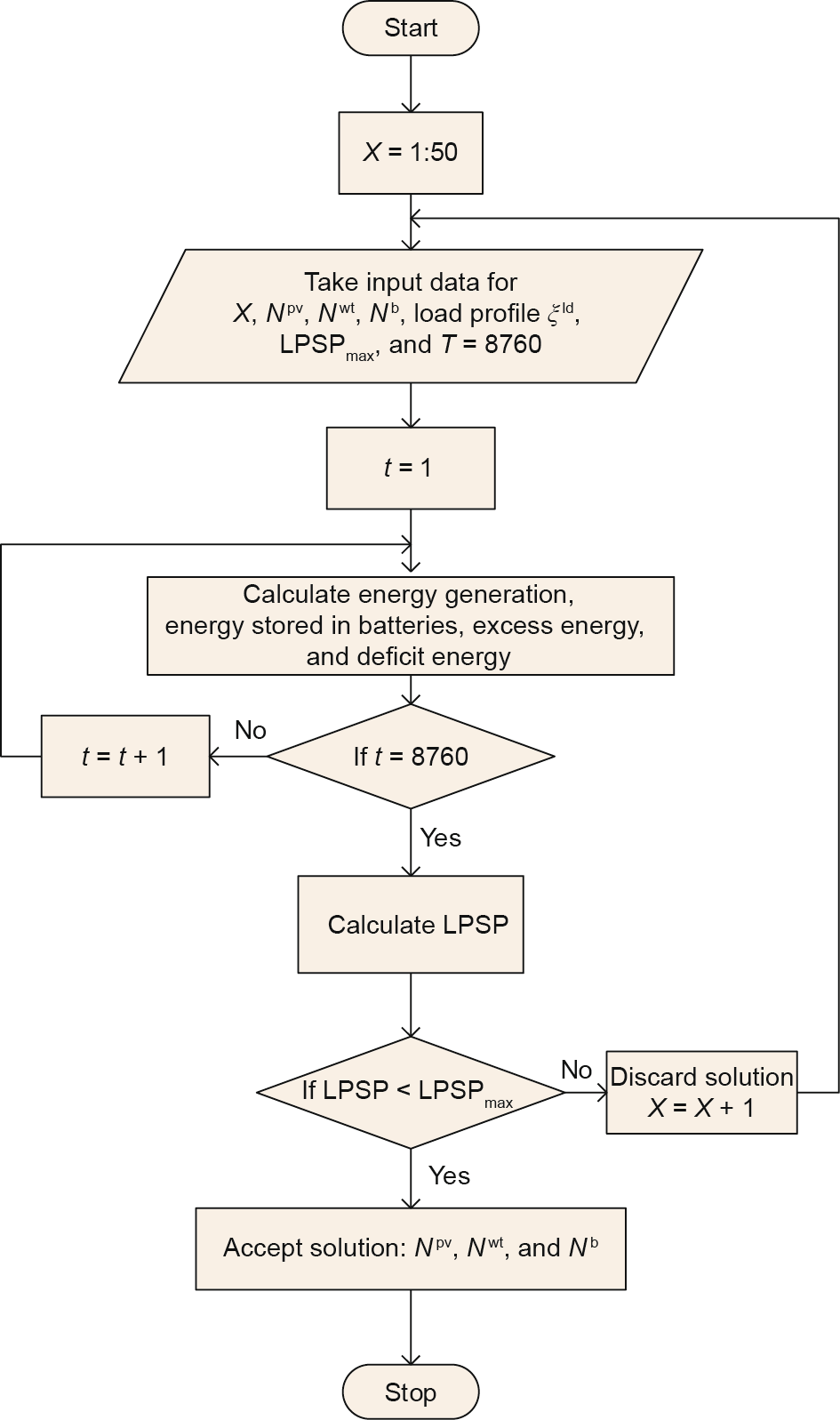
Fig. 2. Flowchart for calculating the hybrid system’s reliability.

《2.5. TAC formulation and constraints》

2.5. TAC formulation and constraints

In this section, an objective function based on the TAC minimization is formulated, along with constraints.

(1) Objective function. The objective function is based on finding the optimum number of components required for the HRES to satisfy the consumer’s load at minimum TAC, expressed as . The TAC is derived using two different costs: the annual capital cost and the annual maintenance cost . The former cost occurs at the start of a project, while the latter cost takes place during the life of the project. Thus, minimization of f tac is given by the following formula:

The initial capital cost needs to be converted to the annual capital cost. To do so, the capital recovery factor (CRF) approach is used. The CRF is obtained by Eq. (16) [19]:

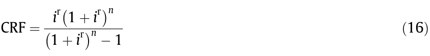
where represents the rate of interest and n depicts the system’s lifespan in years.

everal of the components used in a PV–WT–battery HRES are frequently replaced during the project’s lifespan. For example, the life of the battery is estimated to be five years. Similar to the approach used in Ref. [19], the present worth factor via single payment can be derived using Eq. (17):

where  represents the battery’s present worth and depicts the price of the battery.

Similarly, the lifetime of an inverter/converter is estimated to be ten years. Therefore, the present worth factor via single payment can be defined using Eq. (18):

where  represents the present components’ worth of the inverter/converter and  depicts the price of the inverter/converter. 

Thus, by breaking apart the PV–WT–battery HRES into the annual costs of the PV panels, WTs, battery, and inverter/converter, Eq. (19) is obtained:

where  denotes the WT’s unit cost,  represents the PV panel’s unit cost,  is the unit cost of the battery,  represents the unit cost of the inverter/converter, and  depicts the quantity of the inverters/converters. 

In order to obtain the system’s components’ annual maintenance cost , Eq. (20) is used:

where  and  denote the annual maintenance costs of the PV panels and WTs, respectively. In this paper, the maintenance costs of the inverter/converter and battery units are not considered.

(2) Constraints. The battery bank charge quantity at any time  is subject to the minimum and maximum storage capacity constraint given by the following formula:

where  represents the battery bank maximum charge quantity. The  takes the nominal capacity  value of the battery bank.  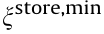shows the battery bank minimum charge quantity, which is calculated by Eq. (22):

where DoD represents the maximum depth of discharge.

In order to have a reliable system, the LPSP constraint given in Eq. (23)(23)is considered during the cost minimization optimization process:

where LPSP_max represents the maximum allowable LPSP value, which is specified by the electricity consumer.

In addition, the following constraints for the total number of PV panels, WTs, and batteries should also be satisfied:

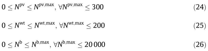
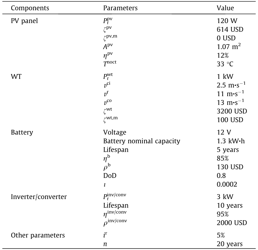
where N ^pv,max , N ^wt,max , and N ^b,max denote the maximum number of PV panels, WTs, and batteries, respectively. In this paper, the minimum and maximum bounds for the decision variables are set at 0–300 for PV panels, 0–200 for WTs, and 0–20000 for batteries. The components and parameters required for the PV–WT–battery hybrid system are given in Table 1 [19]. Fig. 3 provides a schematic diagram of the HRES process based on inputs, processing, and output.

《Table 1》

Table 1 Hybrid system components and parameters.

A^pv : area of the PV panel; : efficiency of the PV panel; : rated power of invertor/convertor; : efficiency of the inverter/converter.

《Fig. 3》

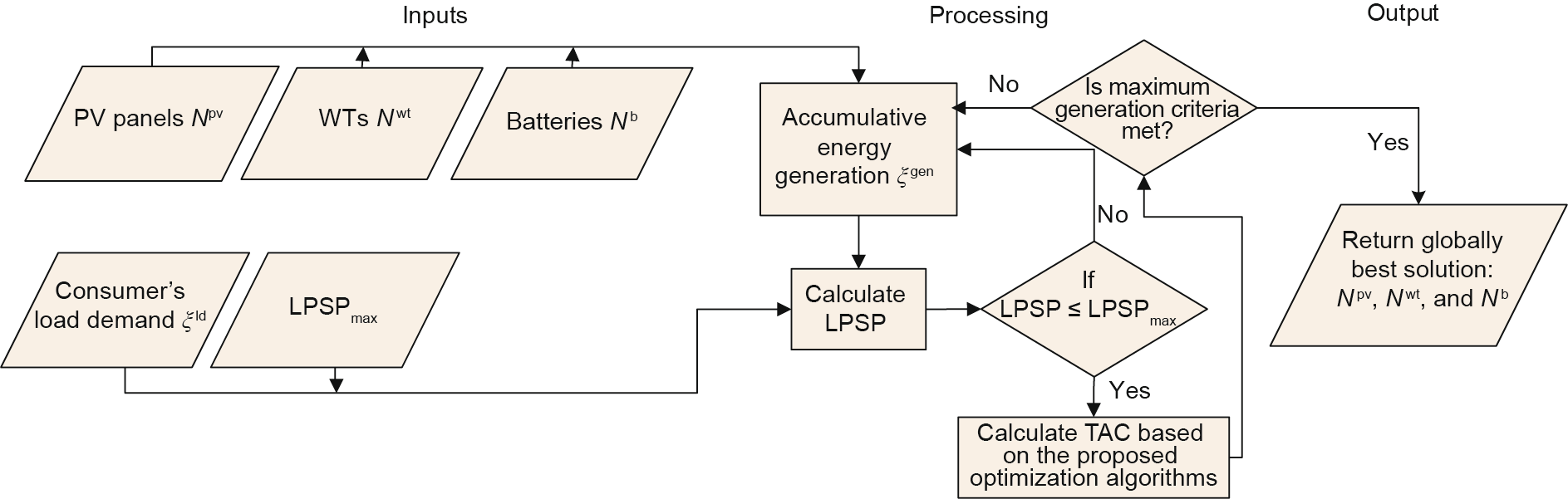
Fig. 3. Schematic diagram of the HRES process.

《3. Proposed methodology》

3. Proposed methodology

Inspired by the use of non-algorithmic-specific techniques, the optimum unit sizing problem is solved using Jaya, TLBO, and hybrid JLBO algorithms; their results are also compared with those of a GA, which requires the algorithmic-specific parameters of crossover and mutation.

《3.1. Jaya》

3.1. Jaya

The Jaya optimization algorithm considers only common control parameters, including population size and termination criteria, and does not require any algorithmic-specific parameters for its execution. In the Jaya algorithm, the objective function is minimized at each iteration i , having the number "c ” of decision variables ( j = 1, 2, ..., c ), and the number "e ” of candidate solutions for a population size (k = 1, 2, 3, ..., e). The best candidate  is selected, which has the foremost value of in the entire solution. Similarly, the worst value of is denoted by , which is assigned as the worst candidate in the entire population. If represents the value of the jth variable for the kth candidate during the ith iteration, then it is changed according to the criteria defined by the following equation [29]:

where  and  are the values of variable j for the best and the worst candidates at the ith iteration, respectively.  depicts the updated value of , while rand_1,j,i and rand_2,j,i denote the two random numbers for the jth variable during the ith iteration in the range from 0 to 1. The expression "rand_1,j,i (O_j,best,i – O_j,k,i )”depicts the inclination of the solution to move toward the best solution, while the expression "rand_2,j,i (O _j,worst,i – O _j,k,i )” shows the tendency to avoid the worst solutions.  is only accepted when it achieves a better fitness value. During the optimization process, accepted solutions are utilized to update the population for the next generation. To avoid negative and decimal values, we used the absolute and floor functions of MATLAB, respectively, to obtain an integer value for the decision variables.

《3.2. Teaching–learning-based optimization》

3.2. Teaching–learning-based optimization

In TLBO, the rows and columns of the population represent the learners and subjects, respectively. Each subject of the learner is related to the decision variable, whereas the total number of subjects of the learner corresponds to a solution. The TLBO process is divided into two different phases: the teacher phase and the learner phase. The former phase shows learning from the teacher and the latter phase is associated with learning via interaction among the learners [30].

In the teacher phase, the mean of the learners is calculated as subject wise. All the learners are evaluated through the fitness function, and the best learner with the minimum TAC will be chosen as a teacher . The algorithm now tries to shift the learners’ mean toward the teacher. Thus, a new vector formed by the current and best mean vectors is added to the existing population, as shown in Eq. (28):

where r represents a random number in the range of 0 and 1, and T_factor is the teaching factor (TF). The TF is selected as either 1 or 2. It should be mentioned that T_factor is not taken as an input parameter; rather, it is randomly decided with an equal probability by the algorithm during the optimization process, as given in the following equation:

and the  in Eq. (28) is only accepted if it provides a better fitness function value.

In the learner phase, each learner randomly interacts with other learners in order to share and increase their knowledge. The process starts by randomly selecting two learners:  and   , from the existing population, such that m ≠ n. Based on the fitness values of the learners, the population is updated by the following equation:

The optimization process of the algorithm continues until some termination criterion is met.

《3.3. JLBO》

3.3. JLBO

JLBO is composed of Jaya followed by the learning phase of TLBO, which results in an increased search power around the global solution. Fig. 4 shows the flowchart of the optimization process of the JLBO algorithm. The mapping steps of the JLBO algorithm to obtain an optimum unit sizing solution for the HRES are given below.

《Fig. 4》

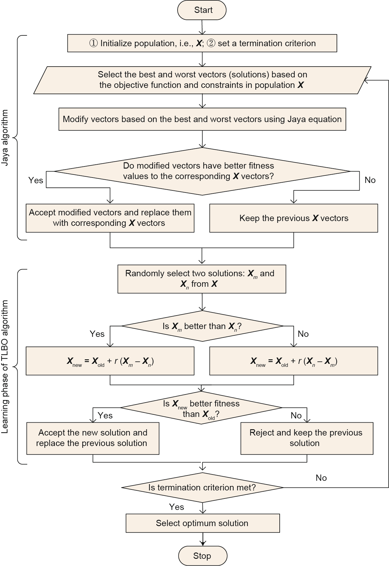
Fig. 4. Flowchart of the JLBO algorithm.

Step 1: The hourly input parameters, including solar irradiation, wind speed, ambient temperature, and consumer’s load profile data, are taken as input.

Step 2: Based on the input data, the power generation capacities of individual PV panels and WTs are calculated via Eqs. (1) and (4).

Step 3: An initial population with the size of 50 is randomly generated, consisting of only two decision variables: X = [N^pv, N^wt]. In this position vector, the first element depicts the total number of PV panels and the second term represents the total number of WTs. To keep the decision variables within the search space, the minimum and maximum bounds (constraints) given in Eqs. (24) and (25) must be satisfied.

Step 4: Here, we calculate the number of batteries for each solution of X using Eq. (12), and apply the constraint given in Eq. (26). X is updated such that it now represents three integer decision parameter values: X = [N^pv, N^wt, N^b ]. Here, the third element corresponds to the total number of batteries. These performance parameters are the decision variables of the unit sizing problem. Thus, the initial population generated now consists of a matrix size of [50 × 3], where 50 represents the rows and 3 depicts the columns for each performance parameter. Each corresponding row of population X depicts a solution to the unit sizing problem.

Step 5: The LPSP of each solution of X is found via Eq. (13). Now only those solutions are considered that satisfy the LPSP_max constraint given in Eq. (23).

Step 6: In this step, the cost values for each solution in X are computed using Eq. (15). Depending on the values of the fitness function, the best and worst solutions in X are now selected.

Step 7: Using Jaya Eq. (27), the first two elements (N^pv and N^wt) of the entire X are updated.

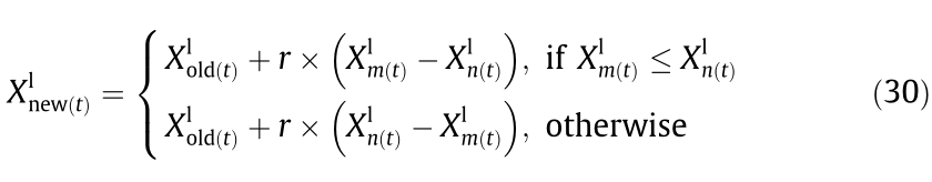
Step 8: During the learner phase, two solutions—X_m and X_n—are randomly selected from X. Based on the fitness function values, X_new is updated via Eq. (30). X_new now contains the updated population values.

Step 9: Finally, Steps 4–8 are repeated until a termination criterion (in this work, 100 generations) is met.

Step 10: The best solution among all generations based on the TAC is selected as an optimal solution, and the corresponding performance parameter values are returned.

《3.4. Genetic algorithm》

3.4. Genetic algorithm

The GA is a bio-inspired algorithm that is dependent on the genetic evaluation and survival of the fittest concepts [35]. The GA has been widely applied to energy management via appliances scheduling [36,37] and unit sizing problems of hybrid systems [38]. In a GA, the algorithmic-specific parameters, including selection, mutation, and crossover operators, are initialized and tuned during the optimization process to achieve a near-optimal global solution. Like other meta-heuristic algorithms, the GA process starts by randomly generating an initial population (X ) with N numbers and D dimensional space. The genes present in the D dimension space represent the decision variables of the problem. In a GA, a chromosome is a complete row consisting of several genes forming a candidate solution to the problem. As the GA optimization process evolves, all chromosomes are evaluated through a fitness function, which is TAC minimization in this study. During an iteration, the best chromosome represents the local best solution (L_best).

To produce a new population (X_new) for the next generation, mutation and crossover strategies are applied. The process repeats and X_new is evaluated through the fitness function. Newer solutions with better TAC are used to replace the previous ones until the termination criterion is satisfied. The best solution with the minimum TAC is selected among all generations as the globally best (G_best) solution. The crossover and mutation values for this study are set to 0.8 and 0.2, respectively.

《4. Simulation results》

4. Simulation results

The simulation results were obtained using MATLAB R2016a software with a system with a 2.9 GHz Intel Core i7 processor with 8 GB of installed memory. A dataset containing hourly data for solar insolation (Fig. 5), ambient temperature (Fig. 6), and wind speed at a height of 10 m (Fig. 7) was obtained for a year (8760 h) from Rafsanjan, Iran [39]. Figs. 5(a)–7(a) and Figs. 5(b)– 7(b) depict the solar insolation, ambient temperature, and wind speed data during the year and during the first 8 d of the year (192 h), respectively. A consumer’s load profile for a year and during the first 8 d is presented in Figs. 8(a) and (b), respectively. The initial charge of the batteries is assumed to be 30% of their nominal storage capacity.

《Fig. 5》

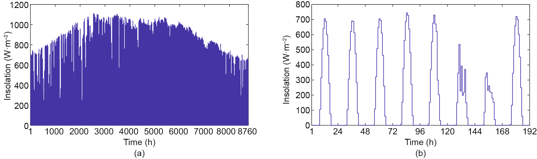
Fig. 5. Hourly solar insolation profile data (a) during a year and (b) during the first 8 d of the year.

《Fig. 6》

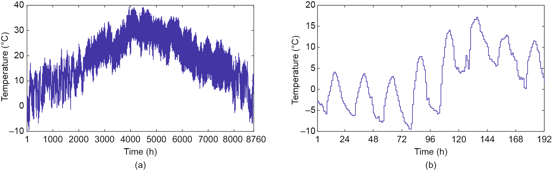
Fig. 6. Hourly ambient temperature profile data (a) during a year and (b) during the first 8 d of the year.

《Fig. 7》

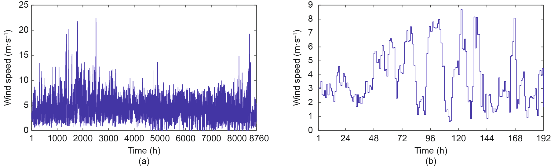
Fig. 7. Hourly wind speed profile data (a) during a year and (b) during the first 8 d of the year.

《Fig. 8》

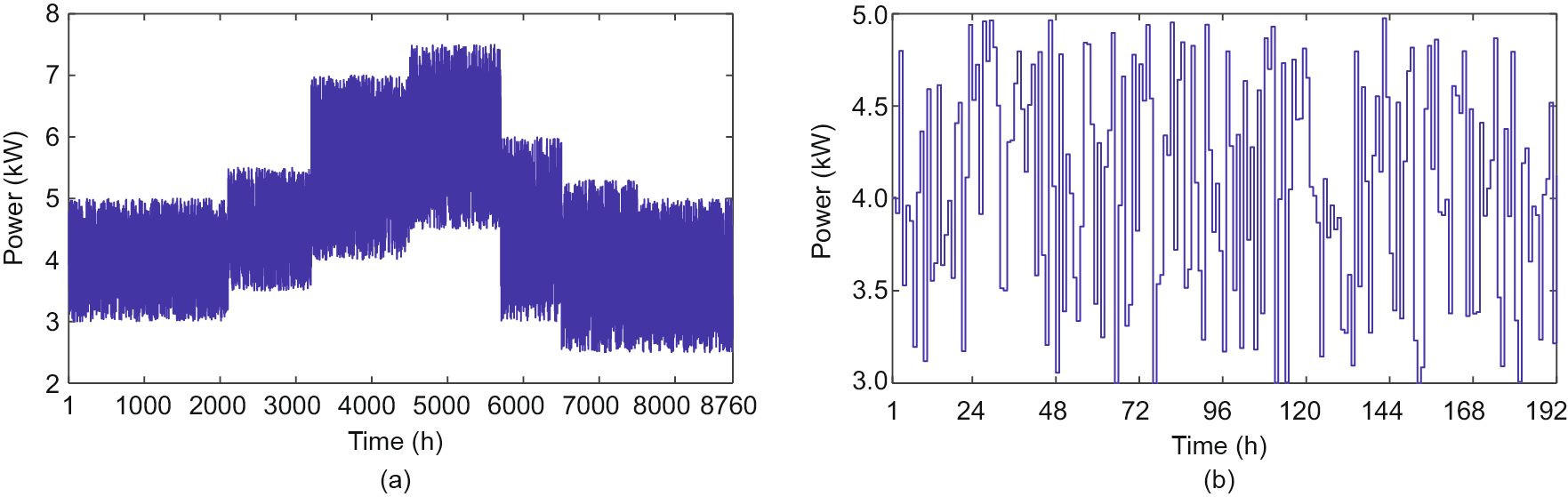
Fig. 8. Hourly consumer’s load profile data (a) during a year and (b) during the first 8 d of the year.

Table 2 summarizes and elaborates the TAC results obtained by algorithms for the optimal sizing of an HRES. In this table, the mean values, standard deviation, and best and worst indexes of each algorithm for all hybrid cases are given. The indexes are reported over ten independent runs. In Table 2, the average rank values of the proposed algorithms are derived by taking the mean of their mean values calculated for all three cases: PV–WT–battery, PV–battery, and WT–battery. For example, the JLBO average rank value 85 183 USD is obtained by taking a mean of 50 247, 67 052, and 138 250 USD achieved by the PV–WT–battery, PV–battery, and WT–battery cases, respectively. The various ranks of the algorithms are assigned based on the average rank of the TACs. As shown in Table 2, the JLBO results show that at LPSP_max = 1%, the PV–WT–battery hybrid system is the most cost-effective solution with a TAC of 50 247 USD, compared with the WT–battery and PV–battery systems with TAC values of 138 250 and 67 052 USD, respectively. The best and worst indexes in Table 2 show the best and worst solutions found by the algorithms during ten independent runs. The standard deviation is defined as a quantity expressing by how much the members of a group differ from the mean value for the group. In Table 2, for the PV–battery, WT–battery, and PV–WT–battery cases, JLBO achieved the same best and worst solutions in ten independent runs; therefore, it resulted in a standard deviation value of 0.

《Table 2》

Table 2 Summary of the mean, standard deviation (Std.), best performance, worst performance, and ranks of the schemes over ten independent runs for the proposed hybrid systems at LPSP_max = 1%.

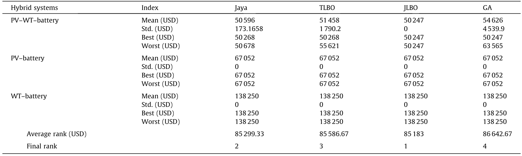
In the case of the PV–WT–battery system listed in Table 2, the optimal sizing that was found for the best index by the Jaya algorithm is N^pv = 160, N^wt = 9, and N^b = 1296, with a TAC of 50 268 USD and an LPSP of 0.9650%. The worst solution found by the Jaya algorithm results in a TAC of 50 678 USD with optimal sizing of N^pv = 155, N^wt = 10, and N^b = 1306 and an LPSP of 0.9340%. The best solution found by the TLBO algorithm is the same as that obtained by Jaya. The worst solution found by the TLBO algorithm achieved optimal sizing of N^pv = 144, N^wt = 13, and N^b = 1453 with a TAC of 55 621 USD and an LPSP of 0.5859%. In the case of the hybrid JLBO, both the best and worst solutions were the same, with a TAC of 50 247 USD, optimal sizing of N^pv = 165, N^wt = 8, and N^b = 1299, and an LPSP of 0.9817%. The best index value obtained using the GA was the same as that obtained using the hybrid JLBO. The worst solution obtained by the GA resulted in a TAC of 63 565 USD with a unit sizing combination of N^pv = 115, N^wt = 20, and N^b = 1682 and an LPSP of 0.8211%.

For the PV–battery and WT–battery systems, all the algorithms achieved the same best and worst solutions, resulting in a standard deviation value of 0. In the case of the PV–battery system, the best and worst solutions resulted in the same TAC of 67 052 USD with optimal sizing values of N^pv = 202 and N^b = 1893 for PV panels and batteries, respectively, and an LPSP value of 0.9715%. In the WT–battery system, we found similar results for the best and worst cases for all algorithms, with a TAC of 138 250 USD and optimal sizing of N^wt = 54 and N^b = 3954. At LPSP_max = 1%, the LPSP obtained by all algorithms was 0.8744%. Therefore, it was revealed that all of the algorithms had a similar performance for the PV–battery and WT–battery systems due to the lower number of decision variables involved in the system, in comparison with the PV–WT–battery system. In the case of the PV–WT–battery system, as the number of decision variables was increased to three (i.e., N^pv, N^wt, and N^b ), the performance of the algorithms varied. The comparative performances of the Jaya, TLBO, JLBO, and GA algorithms at LPSP_max = 1%, showed that the JLBO results were better in terms of mean, standard deviation, and best and worst indexes for the PV–WT–battery system. It is pertinent to note that all the proposed algorithms were evaluated over the same number of generations. The algorithms are therefore ranked as follows based on the fitness values they achieved for the TAC: JLBO, Jaya, TLBO, and GA.

For simplicity, only the results of the Jaya and JLBO algorithms for the proposed hybrid systems are summarized in Table 3. This table provides the optimum results for the decision variables N^pv, N^wt, and N^b in terms of the minimized TAC values at five different LPSP_max achieved by the aforementioned algorithms. It is notable that at all LPSP_max values, the PV–WT–battery system is economical in terms of TAC, in comparison with the PV–battery and WT– battery systems. Due to its enhanced search for more promising areas of the solution space, the hybrid JLBO achieved better results for the PV–WT–battery system. For the PV–battery and WT–battery systems, the results achieved by Jaya and TLBO were similar for all TACs at different LPSP_max values.

《Table 3》

Table 3 Summary of Jaya and JLBO results for the proposed hybrid systems at different LPSP_max values.

N/A: not applicable.

When considering the Jaya algorithm, it was found that at LPSP_max = 0, a TAC of 66 863 USD was achieved with 145 PV panels, 15 WTs, and 1802 batteries for the PV–WT–battery system. As the values of LPSP_max increased from 0 to 5%, the corresponding TAC values decreased due to the tradeoff effect between the cost and reliability of the system. In other words, the system is more reliable but costly and will always fulfill the consumer’s load demand at LPSP_max = 0 as compared with other LPSP_max values, where LOS is probably caused by a lower amount of power generation from the RESs. At an increased value of LPSP_max, that is, at 5%, the PV–WT– battery system achieved the minimum TAC value of 35 555 USD for the Jaya algorithm. An analysis of Table 3 reveals that the PV–WT– battery system provides a more economical solution than the PV– battery and WT–battery systems for the Jaya algorithm. For example, when the LPSP_max value is set to 5%, TAC values of 35 555, 39 409, and 138 250 USD are achieved for the PV–WT–battery, PV–battery, and WT–battery systems, respectively.

Table 3 also reveals that more promising and efficient results are obtained concerning the minimized TAC values by the JLBO algorithm for the PV–WT–battery HRES as compared with the Jaya algorithm. At LPSP_max = 0, the TAC value achieved by the JLBO algorithm is 66 542 USD, which is 321 USD less than that of the Jaya scheme. Here, the optimum sizing found by the JLBO algorithm is N^pv = 150, N^wt = 14, and N^b = 1795. When the LPSP_max value is set at 0.3%, the TAC achieved by the JLBO algorithm is 60 752 USD, which is 350 USD less than that obtained by Jaya. In this case, the optimum size of the components is N^pv = 144, N^wt = 14, and N^b = 1612, with an obtained LPSP value of 0.2962%. At LPSP_max = 1%, the PV–WT–battery system, with a TAC value of 50 247 USD and optimum sizing of N^pv = 165, N^wt = 8, and N^b = 1299, is found to be the most cost-effective HRES in comparison with the PV–battery and WT–battery systems. Here, the total cost saved by JLBO is 21 USD in comparison with the Jaya algorithm. Furthermore, when LPSP_max is increased to 2%, the optimum sizing obtained by the JLBO is N^pv = 168, N^wt = 6, and N^b = 1078 with a TAC and an LPSP of 43 046 USD and 1.7976%, respectively. In this case, the cost saved by JLBO is 20 USD in comparison with the Jaya scheme. Finally, at LPSP_max = 5%, the TAC value found by JLBO is 34 464 USD for the PV–WT–battery system, which is 1091 USD less than the solution obtained by the Jaya scheme. In this case, the optimum sizing of the system components is N^pv = 174, N^wt = 3, and N^b = 818, with an LPSP value of 4.8372%.

As shown in Table 3, the results obtained by the JLBO algorithm for the PV–battery system are more economical in terms of TAC than those for the WT–battery system. The TAC values obtained for the PV–battery system at LPSP_max = 0, 0.3%, 1%, 2%, and 5% are 88 853, 82 790, 76 052, 50 424, and 39 409 USD, respectively. In the case of the WT–battery system, the TAC values obtained are 147 730, 142 150, and 138 250 at LPSP_max = 0, 0.3%, 1%, 2%, and 5%, respectively. The simulation plots obtained by the JLBO algorithm for performance parameters including RESs power generation, status of energy storage in the battery bank, and TAC values along with their convergence are discussed next.

The fulfillment of the consumer’s load at any time instant is mainly dependent on the RES power generation and the extent of energy stored in the battery bank. Figs. 9 and 10 present the hourly produced power by the PV panels and WTs, along with the expected amount of stored energy in the battery bank throughout a year and during the first 8 d of the year, respectively, for the PV– WT–battery HRES considering various LPSPmax values. As depicted in Fig. 9(a), the maximum PV power is produced at LPSP_max values of 5% and 2%, with N^pv of 174 and 168, respectively. The least amount of power produced by PV panels is at LPSP_max = 0.3%, with N^pv = 144. In Fig. 9(b), the highest produced power by WTs has a similar profile for LPSP_max values of 0 and 0.3% because of the equal number of N^wt, that is, 14. The lowest power is produced when the installed number of WTs is 3 at LPSP_max = 5% for the PV–WT– battery hybrid system.

The expected amount of energy stored in the battery bank during a year and the first 8 d of the year is plotted in Figs. 9(c) and 10(c), respectively, at five different LPSP_max values. It is found that a large amount of energy is stored at LPSP_max = 0 because of the large number of installed batteries (N^b = 1795). In this case, the consumer must bear the maximum TAC value of 66 542 USD. As shown in Fig. 9(c), an increase in LPSP_max value results in a decreased amount of stored energy in the battery bank due to the lower number of batteries. For example, at LPSP_max = 0.3%, 1%, 2%, and 5%, the number of batteries N^b is 1612, 1299, 1078, and 818, respectively. Furthermore, loss of load (LOL) is caused at time slots when the amount of stored energy in the batteries reaches the minimum allowable limit.

《Fig. 9》

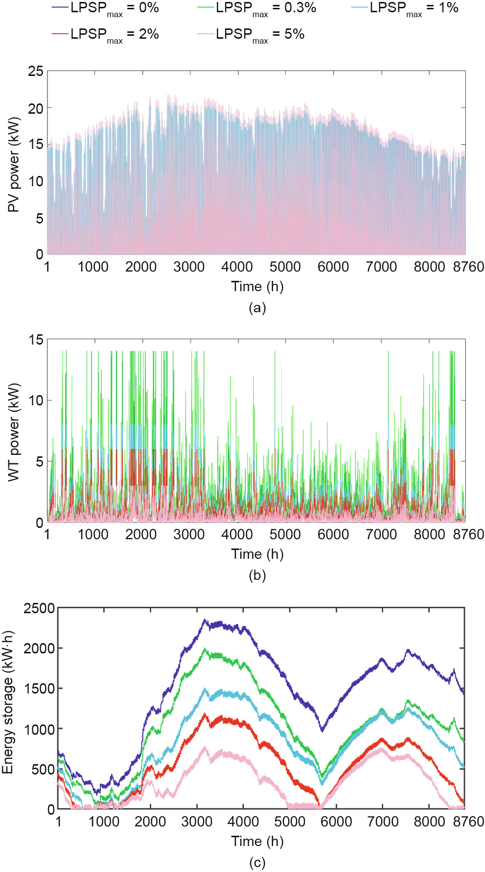
Fig. 9. Hourly produced power and energy storage level of the PV–WT–battery system achieved by the JLBO algorithm during a year at different LPSP_max values. (a) Produced PV power; (b) produced WT power; (c) battery energy storage level.

《Fig. 10》

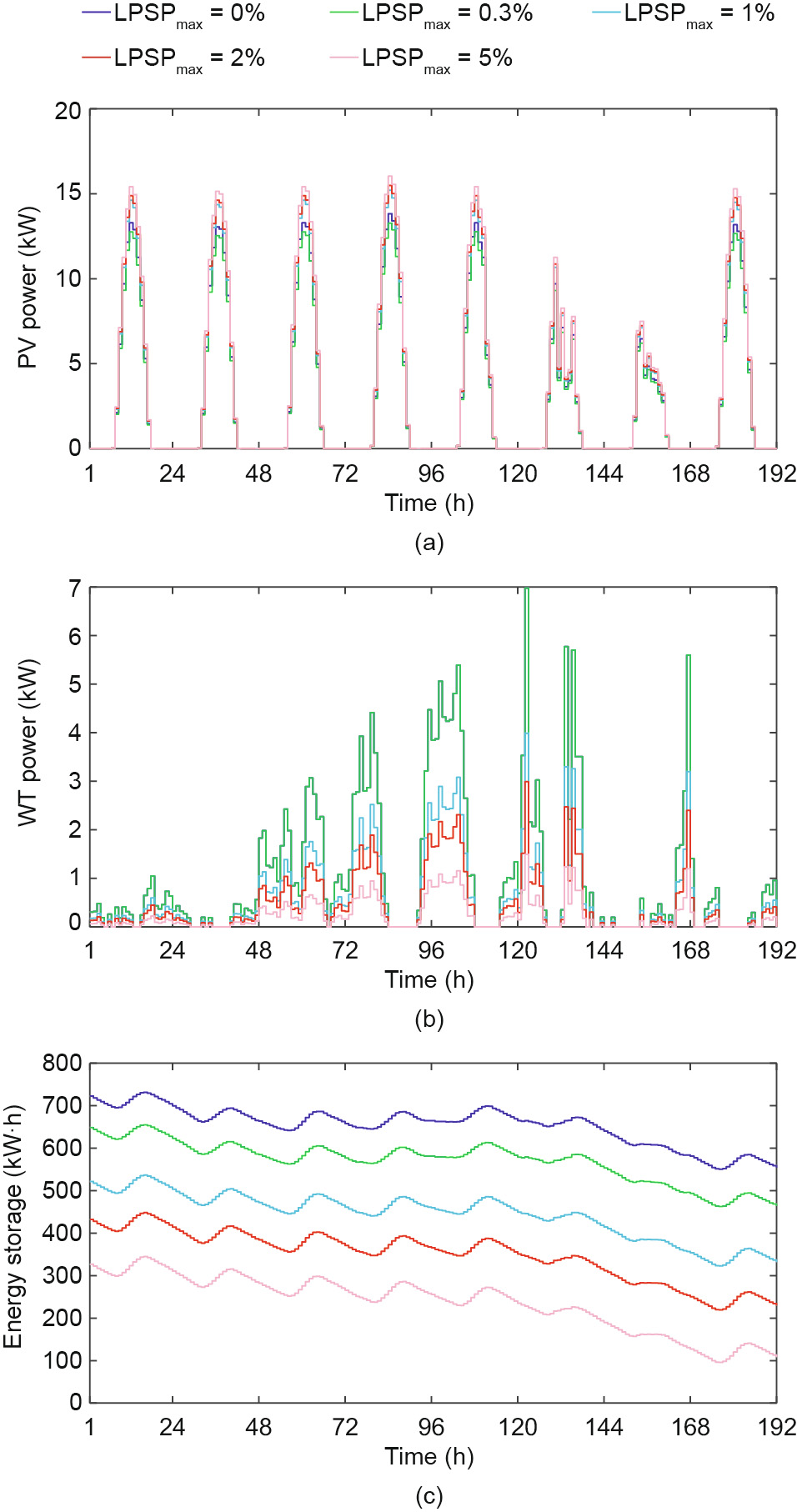
Fig. 10. Hourly produced power and energy storage level of the PV–WT–battery system achieved by the JLBO algorithm during the first 8 d of the year at different LPSP_max values. (a) Produced PV power; (b) produced WT power; (c) battery energy storage level.

The hourly produced PV power and energy storage level of the PV–batteries system throughout a year and during the first 8 d of the year at different LPSP_max values are presented in Figs. 11 and 12, respectively. As shown in Fig. 11(a), at LPSP_max = 0, the hourly produced power is the highest, with 213 PV panels. Accordingly, the consumer bears a maximum TAC of 88 853 USD. When the LPSP_max value increases, there is a relative decrease in the hourly produced PV power, along with the TAC values. At LPSP_max values of 0.3%, 1%, 2%, and 5%, the number of PV panels obtained by JLBO decreases to 210, 202, 193, and 187, respectively. Based on this fact, the amount of power generated by the PV panels is also reduced. The corresponding PV power for the first 8 d of the year is given in Fig. 12(a). Thus, depending on the solar insolation and ambient temperature data profiles, the daily output power of the PV panels varies accordingly.

Fig. 11(b) presents the hourly battery energy storage level of the PV–battery system. As has been already mentioned, it is assumed that the batteries are initially 30% charged. Thus, for different LPSP_max, the starting storage points are dependent upon the number of batteries. For example, at LPSP_max = 0, the PV–battery system results in the highest amount of storage capacity with N^pv = 213 and a TAC value of 88 853 USD. Similarly, a decrease in the expected mass of stored energy is evident with increasing LPSP_max values due to the tradeoff effect between the system’s reliability and the TAC. The stored mass of energy is the lowest at an LPSP_max of 5%, with a TAC value of 39 409 USD. The corresponding energy storage level plot during the first 8 d of the year at different LPSP_max is given in Fig. 12(b). Since the PV–battery system initially utilizes the amount of stored energy in the battery bank due to the lack of renewable power from PV panels, a declining trend in energy storage is observed in Fig. 12(b).

《Fig. 11》

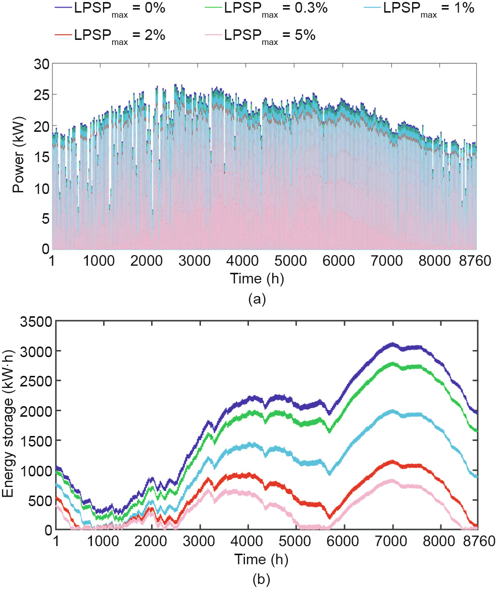
Fig. 11. Hourly produced power and energy storage level of the PV–battery system achieved by the JLBO algorithm during a year at different LPSP_max values. (a) Produced PV power; (b) battery energy storage level.

《Fig. 12》

Fig. 12. Hourly produced power and energy storage level of the PV–battery system achieved by the JLBO algorithm during first 8 d of the year at different LPSP_max values. (a) Produced PV power; (b) battery energy storage level.

Figs. 13 and 14 illustrate the hourly produced power and energy storage levels of the WT–battery system for a year and during the first 8 d of the year, respectively, at different LPSP_max values. The highest power is produced by WTs at LPSP_max = 0, with the maximum number of WTs installed—that is, 56. When LPSP_max is increased to 0.3%, N^wt decreases to 55, resulting in reduced power in comparison with LPSP_max= 0. The power produced by the WT– battery system during the first 8 d of the year at different LPSP_max is given in Fig. 14(a). The profiles depicting the WT–produced power in Fig. 13(a) and the stored amount of battery energy in Fig. 13(b) at LPSP_max values of 1%, 2%, and 5% are similar to those of the same number of batteries and WTs (N^b = 3954, N^wt = 54). Due to this fact, for the aforementioned three LPSP_max values, the TAC borne by the consumer is the same, at 138 250 USD. Similar behavior is observed in the hourly produced WT power and energy storage level of the WT–battery system during the first 8 d of the year in Figs. 14(a) and (b), respectively.

《Fig. 13》

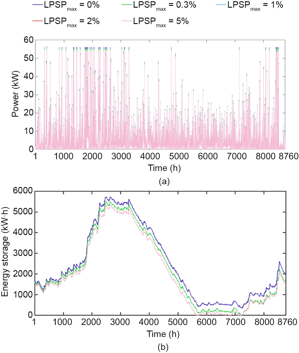
Fig. 13. Hourly produced power and energy storage level of the WT–battery system by the JLBO algorithm during a year at different LPSP_max values. (a) Produced WT power; (b) battery energy storage level.

《Fig. 14》

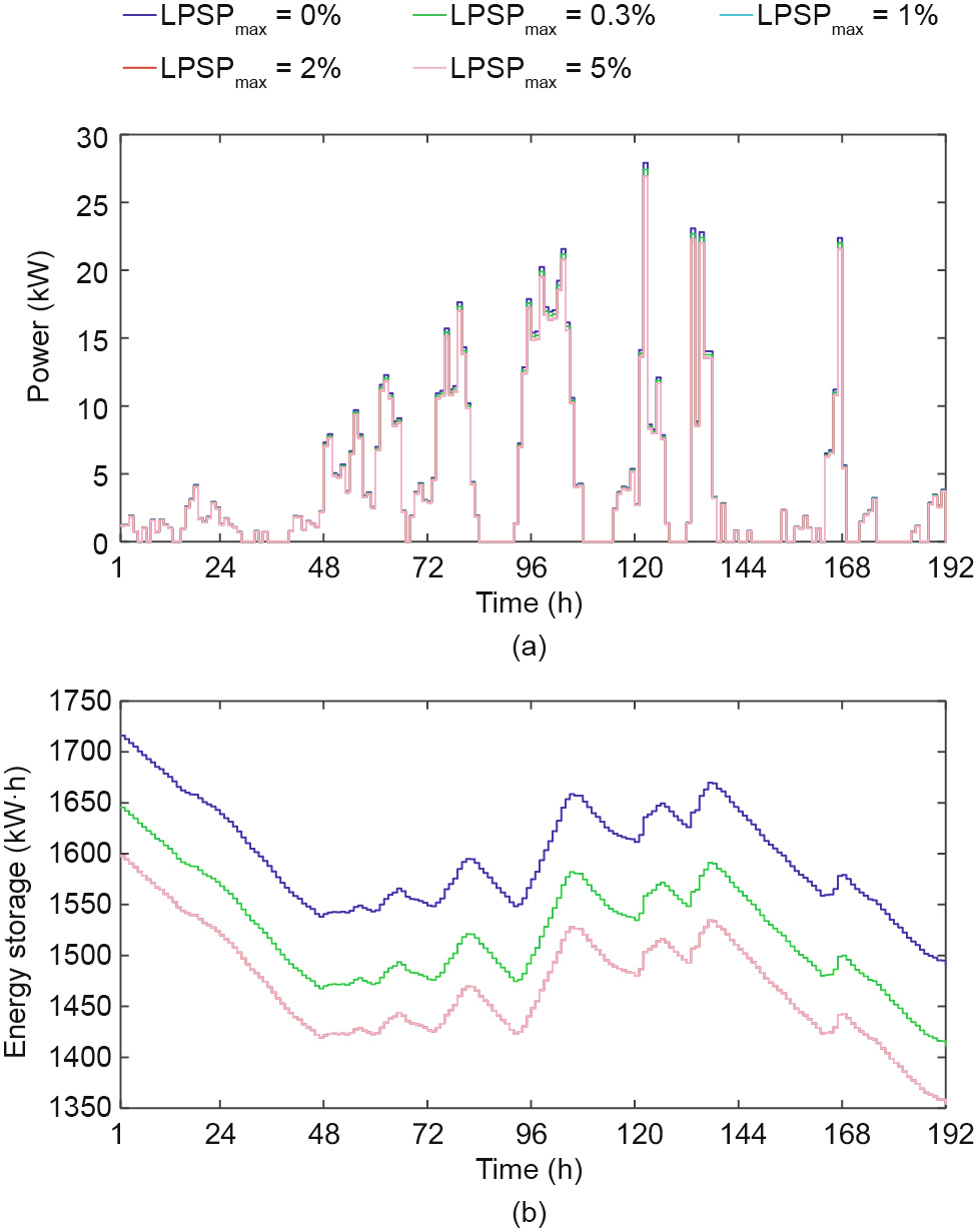
Fig. 14. Hourly produced power and energy storage level of the WT–battery system achieved by the JLBO algorithm during the first 8 d of the year at different LPSP_max values. (a) Produced WT power; (b) battery energy storage level.

Fig. 15 represents the convergence process of the JLBO algorithm while minimizing the TAC of the proposed HRES. It is notable that, at each iteration, the JLBO scheme decreases the TAC value based on the fitness function. This confirms the performance and efficiency of the proposed JLBO scheme for the optimal unit sizing problem. It is also observed that the convergence process of the JLBO algorithm for the PV–battery and WT–battery systems as given in Figs. 15(b) and (c), respectively, is relatively faster than that for the PV–WT–battery system shown in Fig. 15(a), due to the presence of fewer decision variables.

《Fig. 15》

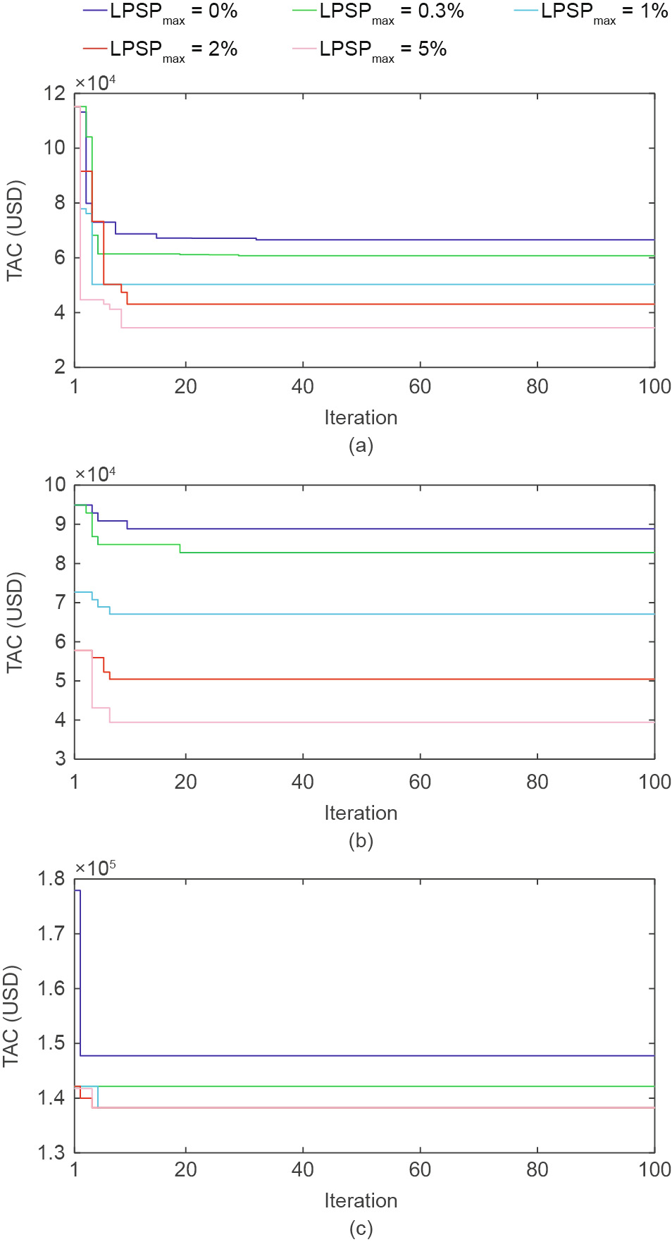
Fig. 15. Convergence process of the JLBO algorithm for obtaining optimum results at different LPSP_max values. (a) PV–WT–battery system; (b) PV–battery system; (c) WT–battery system.

To summarize, it can be stated that the proposed hybrid algorithm JLBO has more promising and cost-effective results than the other algorithms. Furthermore, non-algorithmic-specific parameter schemes, including Jaya and TLBO, are simple because no performance tuning and calibration of their parameters is needed.

《5. Conclusion and future work》

5. Conclusion and future work

In this paper, non-algorithmic-specific parameter schemes were proposed in order to find and evaluate the optimum size of the HRES components required to fulfill the consumer’s load at minimum TAC. To achieve this goal, all components required for the HRES were modeled and a fitness function based on TAC minimization was formulated. The system’s reliability was ensured using various LPSP_max values. To find the optimum unit size of the hybrid system components, Jaya, TLBO, hybrid JLBO, and GA algorithms were applied. When considering the optimization aspect, it was found that the hybrid JLBO algorithm yields more promising and economical results than its ancestors or the GA in terms of the TAC. The PV–WT–battery hybrid system was found to have the most cost-effective solution, with TAC values of 66 542, 60 752, 50 247, 43 046, and 34 464 USD at LPSP_max values of 0, 0.3%, 1%, 2%, and 5%, respectively. The PV–battery system is the secondmost economical solution, and the WT–battery system comes last.

In the future, we are interested in extending this work by comparing it with different meta-heuristic algorithms—including PSO, enhanced differential evaluation, artificial flora, and so forth—that require algorithmic-specific parameters.

《Compliance with ethics guidelines》

Compliance with ethics guidelines

Asif Khan and Nadeem Javaid declare that they have no conflict of interest or financial conflicts to disclose.

《Nomenclature》

Nomenclature

A^pv                          area of the PV panel

CRF                         capital recovery factor

DoD                        depth of discharge of battery

                        objective function in the Jaya algorithm

                    foremost value of in the entire solution

                   worst value of in the entire solution

i                                number of appliances

i ^r                              interest rate

I                                solar radiation

I ^ref                           solar radiation under reference conditions

LOPS                        loss of power supply

LPSP                         loss of power supply probability

LPSP_max                   maximum allowable loss of power supply probability

max(temp)               maximum generation point on the temp curve

min(temp)                minimum generation point on the temp curve

n                               life span of the system in years

N^b                            number of batteries needed for battery bank

N^b,max                      maximum number of batteries

N ^inv/conv                  number of the inverters/converters

N^pv                           number of PV panels

N^pv,max                     maximum number of PV panels

N^wt                           number of WTs

N^wt,max                     maximum number of WTs

O _j,best,i                     Jaya best candidate values of variable j for at ith iteration

O _j,k,i                         Jaya value of jth variable for the kth candidate during the ith iteration

O _j,worst,i                   Jaya worst candidate values of variable j for at ith iteration

p                               appliances power ratings

                          rated PV power

                           nominal power of WT

                    rated power of inverter/converter

POW^pv                      PV panel power output

POW^wt                      WT power

r                                random number

t                                time slot

temp                         temporary storage variable

T ^amb                         ambient air temperature

T ^c                              temperature of PV cell

T ^cof                           PV panels temperature coefficient

T_factor                         teaching factor

T ^noct                          normal operating cell temperature

T ^ref PV                       cell temperature at reference conditions

T ^rsc                            difference between the maximum and the minimum points in the temp curve

                               speed of the wind

                             cut-in wind speed

                             cut-out wind speed

                               rated wind speed

X                                total population size

                             learner m in population X

                             learner n in population X

X_new                          new population generation

                      teacher in TLBO algorithm

                              unit cost of battery

                             present worth of battery

                           annual capital cost

                    unit cost of inverter/converter

                      present components worth of inverter/converter

                           annual maintenance cost

                             unit cost of PV panel

                          annual maintenance cost of the PV panels

                           total annual cost

                            unit cost of WT

                          annual maintenance cost of WTs

                              battery bank charging efficiency

                              efficiency of the inverter

                            efficiency of the PV panel

                     efficiency of the inverter/converter

                                self-discharging state

                           accumulative power generation

                             consumer’s load

                            total produced PV power

                         stored amount of energy in the battery bank

                   battery bank maximum charge quantity

                   battery bank minimum charge quantity

                             total produced WT power

                              battery price

                     inverter/converter price

                              Boolean integer