

《1. Introduction》
1. Introduction
《1.1. Background》
1.1. Background
Building demand flexibility is playing an increasingly important role in ensuring the stability of utility grids, particularly as higher renewable energy penetration is expected in the future [1,2]. Nevertheless, leveraging building demand flexibility involves several critical issues, including flexibility capacity quantification [3], optimal scheduling and control of flexible resources [4], and flexibility development of business modes and markets [5]. Quantifying building demand flexibility is the basis for addressing the remaining problems. It is a great challenge to quantify the demand flexibility of buildings, especially that of residential buildings, due to the usage of various types of household appliances with different flexibility capabilities, operation characteristics, energy usage patterns, and response characteristics. development of business modes and markets [5]. Quantifying building demand flexibility is the basis for addressing the remaining problems. It is a great challenge to quantify the demand flexibility of buildings, especially that of residential buildings, due to the usage of various types of household appliances with different flexibility capabilities, operation characteristics, energy usage patterns, and response characteristics.
In general, the energy demands of residential buildings include space cooling, space heating, and hot water; these demands are mainly satisfied by various household electric appliances such as air conditioners and electric water heaters. The usage of other household electric appliances, including washing machines, clothes dryers, dishwashers, and so forth, also leads to electricity demands. Research has indicated that building load profiles can be adjusted to provide flexibility through demand-side management strategies [6]. The temperature set-points of thermostatically controlled loads—that are, air conditioners, electric water heaters, and refrigerators—can be adjusted to decrease or increase power consumption [7]; the operation time of washing machines, clothes dryers, dishwashers, and so forth can be shifted to off-peak time [8]; and the charging time of electric vehicles can be adjusted [9]. Residential buildings have significant demand flexibility [10,11].
《1.2. Previous reviews》
1.2. Previous reviews
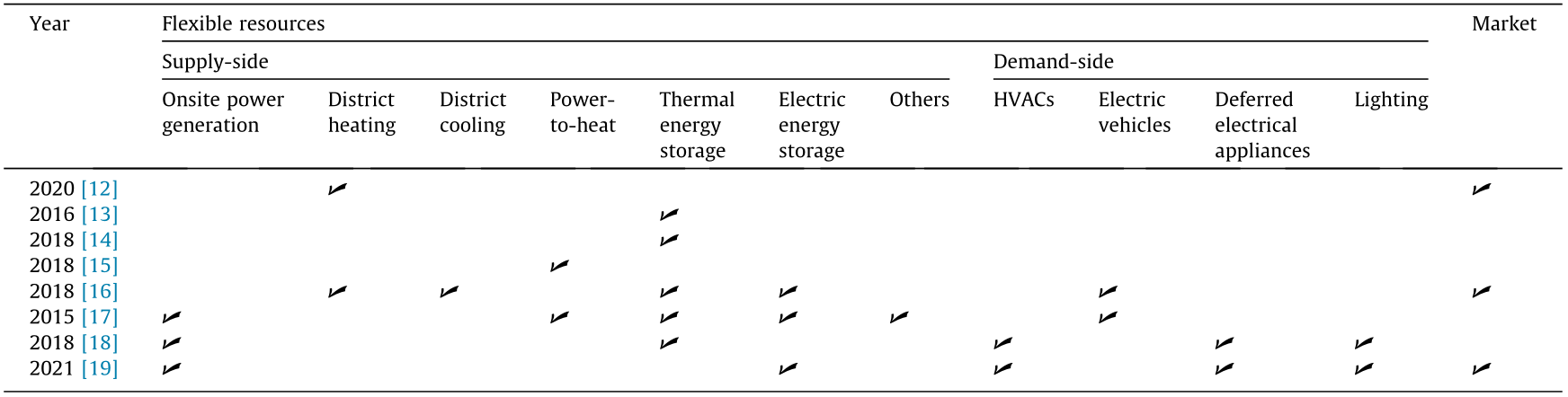
Considerable efforts have been made to quantify the demand flexibility potential of buildings. A review study on energy flexibility in district heating was carried out by Ma et al. [12], which covered the components of district heating systems, markets, and energy flexibility potential. Refs. [13,14] contains reviews of the methods used to evaluate the energy flexibility of buildings, although these methods are not universal and are only applicable to specific systems with certain technologies deployed. Bloess et al. [15] reviewed power-to-heat technologies, modeling approaches, and flexibility potentials for the integration of renewable energy, and concluded that heat pumps and passive thermal storage are particularly favorable options. Moreover, several technological options to improve the flexibility of the Finnish energy system, such as district heating and cooling, electric vehicles, energy storage, smart meters, and demand response, are summarized and discussed in Ref. [16], while a similar literature review can be found in Ref. [17]. However, these reviews [12–17] focus on the supply-side flexibility of building energy systems without considering the load flexibility of end users.
In fact, a few reviews involving building load flexibility have also been carried out. Chen et al. [18] conducted a comprehensive literature review on measures to enhance building demand flexibility. The discussed measures included renewable energy generation; heating, ventilation, and air conditioning (HVAC) systems; energy storage; building thermal mass; shiftable electrical appliances; and occupant behaviors. However, the properties and capabilities of each type of flexible load were not reviewed, and a definition of building demand flexibility, models, and indicators to quantify the flexibility of these flexible resources were not provided. In Ref. [19], different flexible resources in commercial and residential buildings, including building onsite generation technologies, static batteries, HVACs, and shiftable electrical appliances, have been summarized. Nevertheless, reviews on residential flexible loads are limited, as they do not include their characteristics in regard to operation, energy, and time. Moreover, the definition of building demand flexibility and methods to quantify building demand flexibility have not been reviewed.
Table 1 presents a summary of these review articles, which clearly shows that flexibility technologies related to district heating [12,16], district cooling [16], power-to-heat technologies [15,17], thermal energy storage [13,14,16–18], electric energy storage [16,17,19], electric vehicles [16,17], and onsite power generation [17–19] have been well reviewed. The flexibility of residential flexible loads that include HVAC systems, shiftable electric appliances, and lighting has also been investigated in Refs. [18,19]. Nevertheless, reviews on such flexible loads are limited, because these reviews mainly focus on other flexibility technologies. In addition, the definition and quantification methods of building demand flexibility are not reviewed in the above studies. Thus, in order to better comprehend, quantify, and harness residential demand flexibility, it is necessary to perform a comprehensive review of its definitions, flexible loads, and evaluation approaches.
《Table 1 》
Table 1 A summary of review articles on the demand flexibility of buildings.
《1.3. Motivation and work of this paper》
1.3. Motivation and work of this paper
The above literature review shows that the majority of previous review articles on building demand flexibility have been dedicated to overcoming technical hurdles concerning energy utilization in order to improve flexibility potential, while ignoring the flexibility of building demand-side resources. Although some studies have reviewed residential building demand flexibility while considering different types of household appliances, these investigations are limited, as the flexibility capabilities and operation characteristics of these flexible loads have not been clarified well. Furthermore, a comprehensive summary of definitions, models, and evaluation metrics to quantify residential building demand flexibility is lacking.
Therefore, the main purpose of this paper is to conduct a systematic review of the demand flexibility of residential buildings in regard to definitions, flexible loads, and quantification methods. First, an overview of current studies on residential building demand flexibility is given. In order to better understand building flexibility, various terms related to building energy flexibility, operation flexibility, building demand flexibility, and building load flexibility are distinguished. Then, a holistic overview of the definitions of building demand flexibility is presented, and a comprehensive definition is proposed. Moreover, the flexibility capabilities and operation characteristics of the main residential flexible loads are summarized and discussed. The models and evaluation indicators used to quantify the flexibility of these flexible loads are reviewed and summarized, and the research gaps and challenges are identified and analyzed. This review can help readers to better understand building demand flexibility and to distinguish the characteristics of diverse residential flexible loads. This study also provides suggestions for future work on the modeling techniques and evaluation metrics of residential building demand flexibility.
《2. Methods》
2. Methods
This review analyzes in detail those publications focusing on residential building demand flexibility, and was conducted in accordance with the technical roadmap shown in Fig. 1. The keywords used for literature research were divided into three query sets, as shown in Table 2. The three query sets were combined with the ‘‘AND” logic operator for literature research in the Web of Science search engine. The searched articles were then imported into a reference manager to be filtered. First, the searched articles were roughly filtered based on their title, keywords, and abstract, and on the impact factors of their journals. Then, papers relevant to building demand flexibility definitions, residential flexible load characteristics, residential flexible load modeling, and flexibility quantification indicators were picked out after more in-depth reading. Apart from the searched papers, several worthy reports were also downloaded from specific professional websites. The numbers of each type of final selected publication, including review literature, journal papers, conference articles, and reports, are presented in Fig. 2. Finally, the literature review was conducted based on the selected publications; it is composed of four parts, as illustrated in Fig. 1.
《Fig. 1》
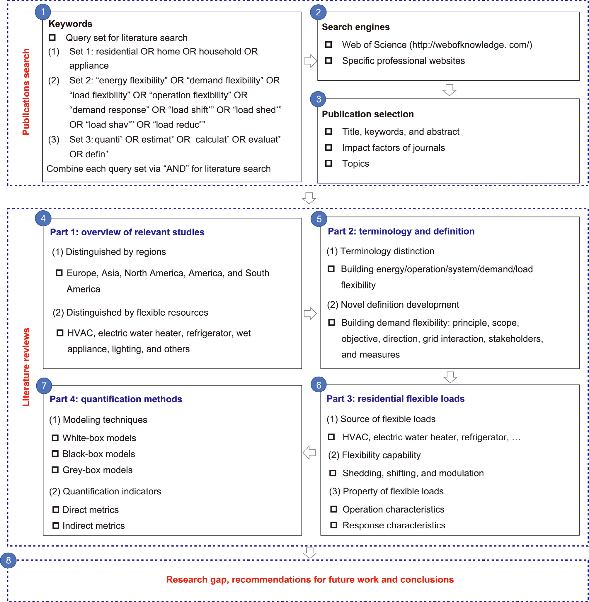
Fig. 1. Technical roadmap of this study. * is the truncation symbol and represents the omitted characters.
《Table 2》
Table 2 Query set for literature search.

《Fig. 2》
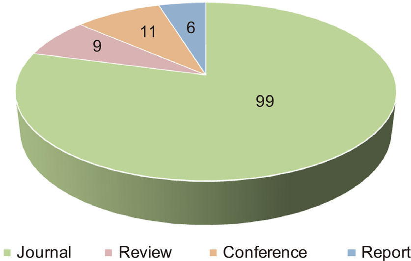
Fig. 2. Numbers of the various types of publications reviewed in this paper.
《3. Overview of studies on residential building demand flexibility》
3. Overview of studies on residential building demand flexibility
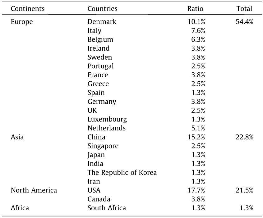
The publications reviewed in this paper have been classified with respect to the authors’ affiliations and research objects, as shown in Table 3 and Fig. 3, respectively. As depicted in Table 3, current research in this field is being led by Europe with 54.4% of all publications. Asia is the continent with the second most publications, accounting for 22.8% of the total publications, followed by North America with 21.5% of the total publications. The remaining continents contribute only 1.3% of the total publications, which are mainly published from Africa. In regard to specific countries, the United States and China investigate residential building demand flexibility the most, producing 17.7% and 15.2% of the total publications, respectively. The United States and China are then followed by Demark, Italy, Belgium, and the Netherlands. In addition to the differences between countries, there are discrepancies in the research objects. As illustrated in Fig. 3, these researchers mainly focus on the flexibility of air conditioners, wet appliances and electric water heaters, for which the proportions are 36.7%, 25.7%, and 14.7%, respectively. Meanwhile, publications on the flexibility of refrigerators and lighting only account for 9.2% and 8.3%, respectively. There are very few studies on other residential flexible loads such as televisions [20]. In particular, regarding the flexibility of air conditioner loads, previous studies have focused on central air conditioning, while the flexibility of packaged air conditioning units has been rarely investigated. Packaged air conditioners are, however, worth studying, especially for China, where packaged air conditioning units are widely used in residential buildings due to the multi-household residential building form.
《Table 3》
Table 3 Distribution of the authors’ affiliations of the reviewed publications.
《Fig. 3》
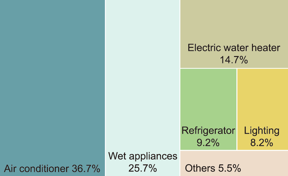
Fig. 3. Distribution of different residential flexible loads investigated in previous studies.
《4. Definition and features of building demand flexibility》
4. Definition and features of building demand flexibility
《4.1. Different terms about building flexibility》
4.1. Different terms about building flexibility
As defined by the Oxford English Dictionary, flexibility is ‘‘the ability to change to suit new conditions or situations.” The first introduction of flexibility to power-system engineering dates back to the 1990s [21]. Since then, this concept has gradually been applied to the fields of energy and buildings, especially to gridinteractive efficient building [22,23]. Nevertheless, to our best knowledge, there is still no unified definition of flexibility, whether for the power-system field [24,25] or the building energy conservation field [26–28]. Several terms associated with the flexibility of buildings, including energy flexibility, demand flexibility, load flexibility, and operation flexibility, have emerged but have not been clearly distinguished when used. In some reports [23,29], the authors seem to imply that the energy flexibility, demand flexibility, and load flexibility of buildings are the same. One report [29] defined building demand flexibility as the capability of distributed energy resources to adjust a building’s load profile across different time-scales, and stated that energy flexibility and load flexibility are often used interchangeably with demand flexibility. In many studies [8,30–32], the demand flexibility, operation flexibility, and energy flexibility of buildings have uniform implications. As far as we can see, it is reasonable for the terms demand flexibility and load flexibility to have the same meanings. However, terms such as the energy flexibility, demand flexibility, and operation flexibility of buildings have different meanings from the perspective of the building. A systematic distinction of these terms is expressed in Fig. 4 and described in detail as follows.
《Fig. 4》

Fig. 4. Distinction of various terms used to describe the flexibility of buildings.
Building energy flexibility covers the widest range among the four terms. It contains all flexible resources of a building, including building energy systems, the building itself (e.g., envelope, HVACs, electric appliances, and electric vehicles) as well as the occupants’ behaviors [33]. At the supply side of a building energy system, distributed energy generation (e.g., solar photovoltaics (PVs); wind turbines; and combined cooling, heating, and power) is popularly deployed to decrease the building’s net load imported from the utility grid. Hence, numerous researchers believe that a building’s onsite generation can contribute to building energy flexibility [18,19,34,35].
Moreover, integrating various technologies can enhance the flexibility of a building energy system operation, which is known as operation flexibility [36] or system flexibility [37]. Ref. [31] has demonstrated that the combination of utility grids and district heating networks can improve the flexibility of space heating. Furthermore, integrating building energy systems and energy storage systems can improve the operation flexibility via optimized charging and discharging [38–40]. Operation flexibility can also be enhanced by employing advanced technologies such as powerto-gas and power-to-hydrogen in energy systems [17,41].
For the demand side, some building loads such as HVACs, electric appliances, and electric vehicles can be shifted, curtailed, or moderated to a degree through various demand-side management measures [42–44]. This is known as building demand flexibility or building load flexibility. Therefore, the energy flexibility, demand flexibility, and operation flexibility of buildings have different meanings and application scopes.
Building energy flexibility includes supply-side flexibility and demand-side flexibility. The former is further divided into generation flexibility and operation/system flexibility. Generation flexibility is rooted in the flexibility of building onsite generation technologies that reduce the building’s net power, while operation flexibility describes the flexibility of building energy systems operation. Demand-side flexibility (or load flexibility) refers to the flexibility of building loads derived from different energy-using appliances. A systematic distinction of these terms makes their implications much clearer and avoids confusing usage in future. It can also help readers to better understand and distinguish various types of building flexibility
《4.2. Definition of building demand flexibility》
4.2. Definition of building demand flexibility
The terms energy/demand/operation flexibility are distinguished above from the perspective of flexible resources. Nevertheless, distinguishing between them does not answer the question, ‘‘what is building energy/demand/operation flexibility?” Currently, numerous definitions related to these terms exist, and there is no commonly agreed-upon standard definition. In this paper, we focus on building demand flexibility. A holistic overview of the definition of building demand flexibility is presented and a comprehensive definition is proposed in this section.
The diverse definitions of building demand flexibility in the previous literature are summarized in Table 4 [1,8,19,23,45–47]. Since the meanings of building energy flexibility and building demand flexibility are not distinguished in many papers, the definitions of building energy flexibility are also listed in Table 4. It is clear that the most common idea behind building flexibility is to adjust a building’s loads to satisfy various requirements, such as user needs, surrounding energy-network requests, and grid requirements. However, the majority of definitions are either somewhat unclear or somewhat narrow in their scope and are quite casespecific. Moreover, most definitions do not clearly show the principle that the usage of building flexibility does not sacrifice occupant comfort, productivity, and health, as these definitions are proposed only from the perspective of one stakeholder—either the grid operators or building owners. Considering these limitations, a more comprehensive definition of building demand flexibility is proposed in this study. Building demand flexibility is defined as the ability to manage a building’s flexible resources in order to change its load profile to meet different requirements without sacrificing end-user interests. In this definition, the requirements are to curtail a building’s peak load, flatten the building power-consumption curves, improve renewable energy self-consumption, maintain energy-network stability, provide grid services, reduce end-user energy costs, and so forth. The interests of end users include their comfort, productivity, health, and convenience. The proposed definition has a much wider application scope, as it can be applied to heating supply networks, power networks such as utility grids and microgrids, and so forth. It can also be applied to various building types, such as commercial buildings and residential buildings.
《Table 4 》
Table 4 Definitions of building energy flexibility and building demand flexibility.

In this paper, we focus on the application of residential demand flexibility in power networks. Although the definition is developed for building demand flexibility, it can be extended to building energy flexibility when the scope presented in the definition consists of all the flexible resources of the building. Table 5 provides a comparison between the strengths of the proposed definition and those of the definitions provided in previous studies. It can be seen that the proposed definition is more explicit and comprehensive, with a wider application scope.
《Table 5》
Table 5 Comparison of the strengths of the proposed definition with those of previous definitions.
《5. Flexible loads in residential buildings》
5. Flexible loads in residential buildings
Residential buildings generally contain numerous household electrical appliances. As presented in Fig. 5, a residential building usually contains seven categories of electric appliances: cold, heating, wet, cooking, lighting, brown, and electric vehicles [48,49], although these categories may vary in different countries [50]. Residential buildings can provide demand flexibility for utility grids through load shifting, load shedding, and load modulation such as frequency regulation and voltage support [29]. Previous studies have concentrated on the flexibility of central air conditioners, electric water heaters, wet appliances, refrigerators, and lighting, as shown in Fig. 3. Therefore, the flexibility capabilities and operation characteristics of these flexible loads are clarified in detail in the following sections.
《Fig. 5》
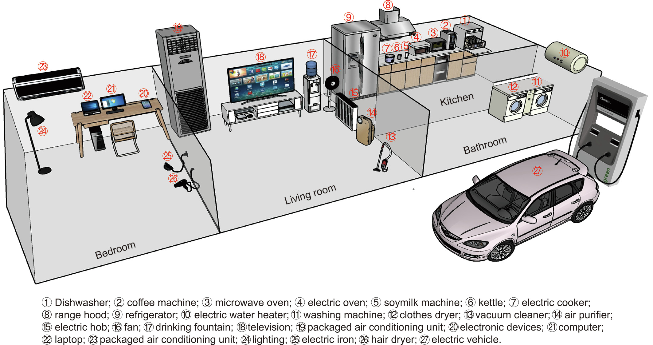
Fig. 5. Household electrical appliances that might be found in a typical residential building.
《5.1. Heating, ventilation, and air conditioning》
5.1. Heating, ventilation, and air conditioning
HVAC systems are vital and unique building flexible loads, accounting for 40% of building energy consumption and contributing significantly to building peak demands in summer and winter [51]. They usually operate intermittently in summer and winter to maintain the indoor temperature, humidity, and CO2 concentration within the desired ranges in order to guarantee the occupants’ comfort, productivity, and health [52].
Common measures by which HVAC systems provide demand flexibility for utility grids include temperature set-point resetting and pre-cooling/pre-heating. By increasing the room temperature set-point, the air conditioning load can be shed during summer peak time; however, this will lead to a rebound effect, because the room temperature needs to be restored to the original value, as illustrated in Fig. 6(a). Moreover, pre-cooling/pre-heating is a promising demand-side management measure that leverages the thermal inertia of a building’s elements, such as its envelope (e.g., exterior walls and roof), indoor air volume, and indoor thermal mass (e.g., furniture and interior walls) [53,54], without downgrading occupant comfort. Cooling/heating capacity can be stored in a building’s thermal mass by HVAC systems and then discharged during the peak demand period to provide load shifting and shedding services for utility grids, as shown in Fig. 6(b). In addition to providing peak demand reductions, an HVAC system can provide load-modulation services through the strategies of static pressure adjustment, water-supply temperature resetting, and frequency control [51]. HVAC systems can provide load shedding, load shifting, and load-modulation services [51,55,56].
《Fig. 6》
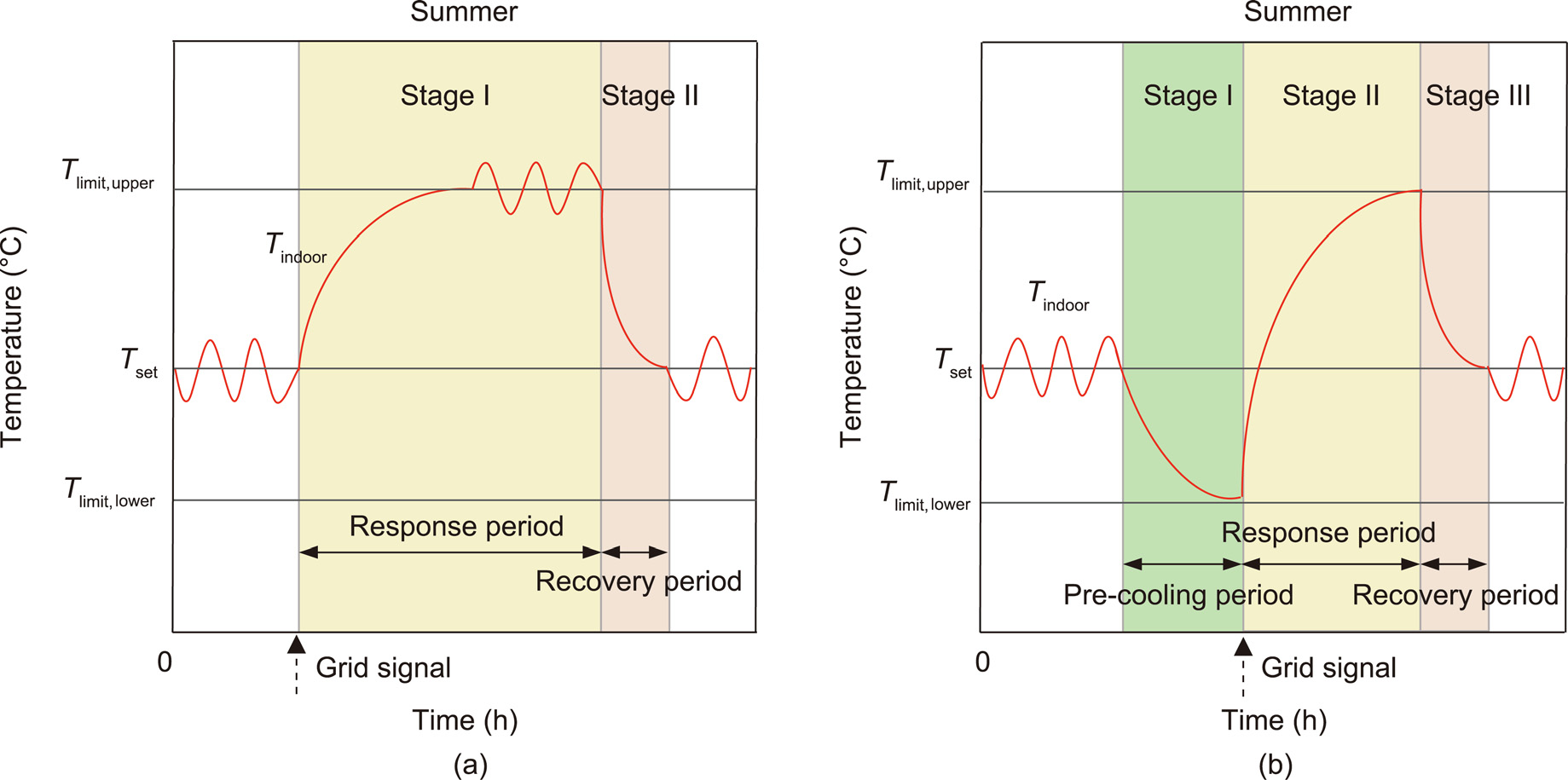
Fig. 6. HVAC demand response: (a) global thermal zone temperature reset; (b) pre-cooling. Tset is set-point temperature of HVACs; Tlimit,upper and Tlimit,lower are the upper limit and lower limit of thermal comfort temperature range, respectively; Tindoor is indoor air temperature of rooms.
In general, HVAC systems under various demand-side management strategies have diverse response characteristics in regard to response time, ramping time, response duration, and load shifting and shedding potential. As summarized in Table 6, under a setpoint adjustment strategy, an HVAC system usually responds in less than 2 min and ramps for 5–30 min, with the curtailment period lasting for 0.5–4.0 h to decrease the peak loads of the grid. The response duration under a pre-cooling/pre-heating strategy is 0.5–3.0 h, but the response time and ramping time are not clear. To provide frequency regulation, the response time of an HVAC is usually less than 1 min, and the response duration is from seconds to minutes. The response characteristics of HVACs depend on several factors such as communication delay, mechanical response delay, or system inertia delay, and these factors vary for different HVAC systems [57]. At present, the majority of studies on the flexibility of HVACs are conducted using simulation software, including TRNSYS [26,58], EnergyPlus [55,59–61], Dymola [35], GAMS [62], and some software combinations [63,64], as well as some datadriven approaches [42,56,65]. Nevertheless, it is difficult to explore the response characteristics of HVACs through these ways alone, as a more comprehensive investigation requires experiments. Moreover, various flexibility potentials under different strategies have been obtained in previous studies. However, it is difficult to compare the various flexibility potentials with each other due to inconsistencies between the studies in regard to, for example, the type of HVAC system studied, the boundary conditions enforced, and the evaluation indicators adopted.
《Table 6》
Table 6 Response characteristics of HVAC loads.

《5.2. Electric water heaters》
5.2. Electric water heaters
Electric water heaters are typically available in two primary configurations: storage and tankless [51,73]. An electric storage water heater is capable of shedding and shifting loads. Water heaters with storage capability that heat the water inside a container and then store it for later usage are employed in many residential buildings. Such heaters usually work intermittently to maintain the water temperature within desired temperature bounds that are typically set differently in various seasons.
The water temperature rises when the electric water heater operates and falls when the appliance is turned off, due to hotwater consumption or standby heat loss [74,75]. The temperature set-point and upper/lower limits are determined by the end user; hence, they vary from one occupant to another. Electric water heaters can provide load-shedding and load-shifting services [51], which are impacted by the occupants’ preferences in water temperature and tolerable temperature range [76]. As with HVAC systems, building owners can decrease the water setting temperature to reduce electricity consumption during the peak time, with little impact on the occupants. This action also reduces the standby heat losses of hot-water storage systems [68]. Once the curtailment period ends, electric water heaters operate in a higher power mode to heat the water temperature to the setting value [8]. Pre-heating is also a popular demand-side management measure for electric water heaters to shift loads away from peak demand periods, which is similar measures for HVAC systems. However, preheating increases the standby heat losses of hot-water storage units [77]. Electric water heaters can also provide loadmodulation services covering frequency regulation, synchronous reserves, and so forth [78].
Some research has been done on the flexibility of electric water heaters. For example, D’hulst et al. [8] estimated the flexibility potential of an electric water heater with a rated power of 2.4 kW based on data obtained in pilot tests. According to their results, the maximal power curtailment of an electric water heater was 0.3 kW, which could be sustained for more than 10 h during the day. To provide different grid services in regard to peak shaving, frequency regulation, synchronous reserves, and so forth, a novel electric water heater model was developed [78] that incorporates both thermal losses and water usage to determine the water temperature in the tank. A voltage-control strategy was proposed to manage aggregated residential electric water heater loads in order to reduce peak demands [79]. In Ref. [80], the scheduling of an electric water heater on a typical day was optimized in order to minimize electricity costs while maintaining the water temperature within the desired comfort range. Similar studies [81–84] also exist. Electric water heaters have also been used to match the residential PV power generation [73]. Electric water heaters are a vital flexible resource on the residential building demand side and can be used to shed, shift, and modulate loads to maintain utility grid stability. However, their response characteristics under different demand strategies remain unclear, since studies on this topic are rare [85].
《5.3. Refrigerators》
5.3. Refrigerators
Refrigerators are widely used in residential buildings and can offer demand flexibility to utility grids [32,51]. Similar to HVAC systems, refrigerators run a vapor compression cycle to transfer the heat from the internal space to the external environment [86]. They operate intermittently to maintain the refrigerated cavity within specific temperature bounds, thereby preventing food spoilage [87]. Refrigerators can provide utility grid services through low-power-mode continuous operation for load shifting [51] and set-point resetting for load shedding [88]. They can also provide load-modulation services [89]. As stated in Ref. [90], a refrigerator can respond to power requests for less than 30 s, and can maintain consumption adjustment for 15 min to regulate frequency and for 1 h to provide load-shedding services by modifying the internal temperature set points. The response characteristics of refrigerators have rarely been investigated in other studies. The flexibility of refrigerators with phase-change materials was exploited to decrease peak loads and running costs by optimizing a refrigerator’s cyclic operations under time-of-use tariffs [91].
《5.4. Wet appliances》
5.4. Wet appliances
Wet devices, also known as white goods [92], are promising flexible loads. These devices include dishwashers, washing machines, and clothes dryers, and account for 15% of total household demand. In general, these appliances operate in finite cycles that are usually started manually by the occupants according to their needs. Once these devices start up, they are not normally shut off until the finite cycle has ended. The finite cycle of wet appliances has a fixed duration. Nevertheless, different views still exist; for example, the authors of Refs. [82,93] divided the operation of wet appliances into a set of sequential energy phases, in which adjacent stages can be interrupted.
Wet appliances provide demand flexibility through the occupants delaying or advancing the start of these appliances in order to shift the entire cycle away from peak demand periods, with few effects on usage. However, these appliances have no loadshedding capability, as their cycles can only be run at different times while their total energy consumption remains constant. Thus, these devices cannot provide any load-modulation services. The demand flexibility of wet appliances is determined by their usage frequencies: The more frequently they are used, the greater the flexibility they provide. In real life, dishwashers may be used twice a day or once a day. Washing machines and clothes dryers may be used every day in summer and less frequently in winter. The usage frequency relies on the occupants and varies from individual to individual depending on age, gender, living habits, population, and income [94,95]. The usage frequency is also different on weekdays and weekends, as well as in different seasons [8,50]. To quantify the shifting flexibility capacity of wet appliances, the concept of a ‘‘flexibility window,” (twindow) which is defined as the duration between the configuration time and the deadline, was proposed by D’hulst et al. [8]. The flexibility of wet appliances in the time window is illustrated in Fig. 7. According to the relationship between twindow and the duration of peak demand, tpeak, different flexibility potentials can be obtained. From Figs. 7(c–f), it can be seen that the loads of wet appliances can be partially shifted away from peak demand periods; under the conditions shown in Figs. 7(a), (b), (g), and (h), they can be shifted completely. The flexibility of wet appliances depends on the setting of the flexibility window.
《Fig. 7》
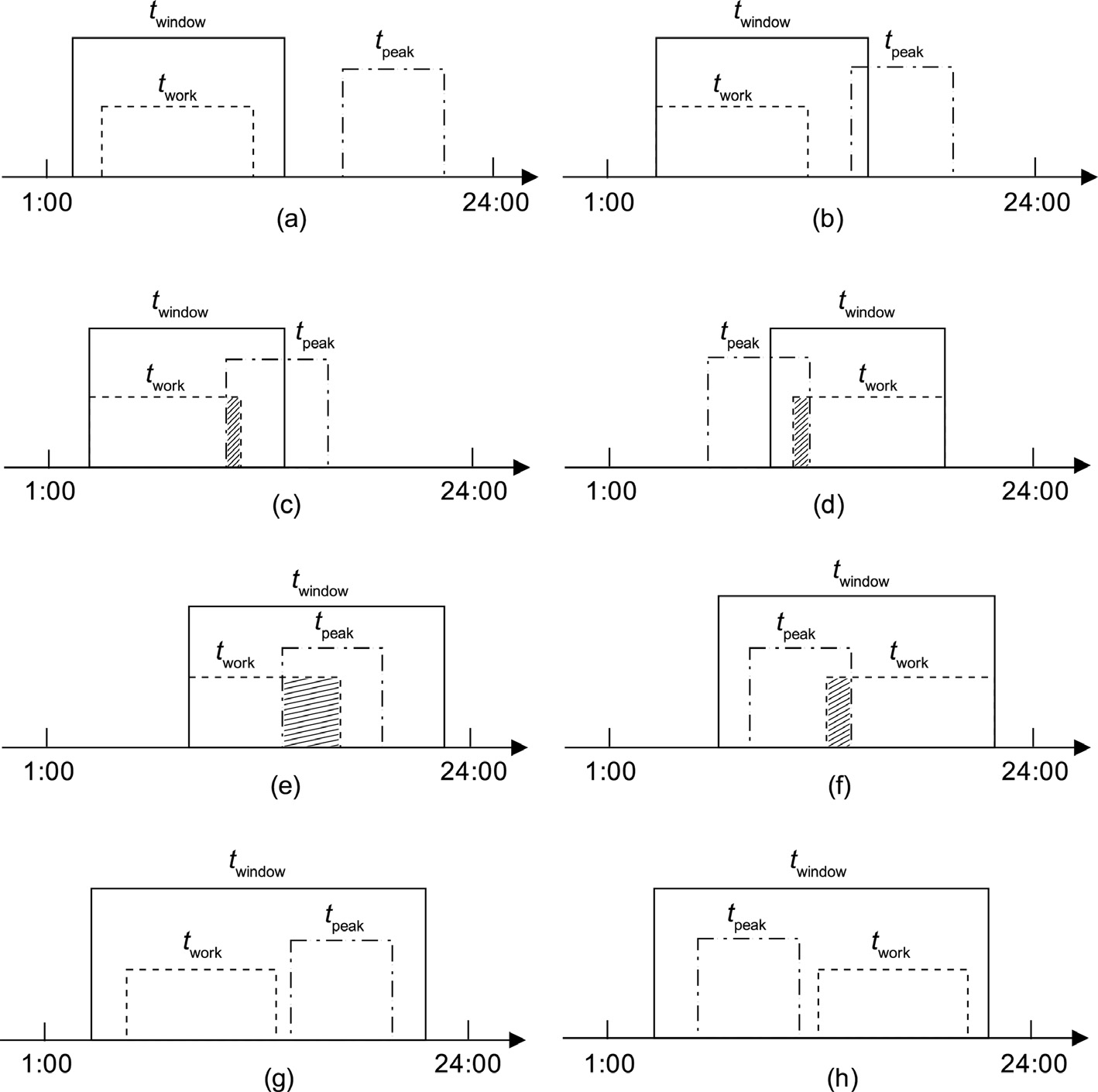
Fig. 7. Load flexibility of wet appliances. twork: the duration of appliance working.
Previous studies have investigated the flexibility of wet appliances in detail, focusing on the evaluation of the demand flexibility of wet devices [8,30,50,93,96–102] and the benefits of wet-device load shifting [46,81,82,97,103–107]. Different ways of tackling these problems, including experiments [8,50,92,97–102,104,107], simulations [81,82,93,103,106,108–111], surveys [30], and an integration of experiments with simulations [96,105], have been employed. The common way to assess the flexibility of wet appliances is to analyze their potential based on the measured data in pilot tests [98–101]. First, probabilistic models of consumer behavior are established. Then, the households participating in the experiment are divided into different groups. Lastly, the flexibility profile of each group is calculated using statistical methods. These processes are essential for estimating the flexibility potential of wet devices at a national level [8,30,50,93,96, 102]. These studies have reached a few common conclusions. Wet appliances have significant load-shifting potential, which is higher on weekends than on weekdays, is higher in winter than in summer [8,50,101,102], and can be stable over a long period of time [99,100]. Moreover, the load-shifting flexibility of dishwashers is much higher than that of washing machines [30,98,101]. To benefit from the load shifting of wet devices, a single-objective optimization model is usually deployed to optimize the starting time of wet appliances, with the aim of minimizing energy costs within a specific electricity tariff. In this model, the usage patterns of wet appliances are obtained through experiments [104,107], simulations [81,82,106,108–111], and the integration of experiments with simulations [96,105]. According to these studies, the load of wet devices can be shifted to a time when the electricity price is low, with the self-consumption of local power generation increasing and electricity costs decreasing.
《5.5. Lighting》
5.5. Lighting
Lighting is considered to be a flexible load; it accounts for 10% of the total energy consumption of residential buildings [112] and can rise to 15% for commercial buildings [113]. Lighting systems are widely used in buildings to maintain an adequate level of visual comfort for the occupants and function in conjunction with natural daylight to achieve this comfort. Lights are mainly used at night and tend to run continuously, only being switched off when the occupants sleep or leave. Lighting loads depend on weather conditions, the geometry of buildings, and occupancy profiles [114,115]. When there is sufficient daylight to satisfy the need for indoor lighting, artificial lighting can be turned down without jeopardizing the occupants’ visual comfort [114,116]. For example, when the indoor illumination is above 500 lx in a residential room, the lighting can be switched off through the energy management system [117]. Therefore, lighting systems can provide demand flexibility by shedding loads. In contrast to other flexible loads such as HVACs and wet appliances, lighting demands cannot be shifted. Moreover, lighting systems can respond quickly to provide grid ancillary services without delay, compared with other household electric devices [19]. The flexibility of lighting loads is time independent, since indoor illumination at a certain moment is only relevant to the current lighting power and is not impacted by the lighting situation at an earlier point in time.
Dimmable lighting systems have been increasingly employed in modern buildings in the past few years. The illumination of such systems can be adjusted to maintain good visual comfort [118]. In Ref. [35], three different dimming levels were adopted to quantify the flexibility potential of lighting during peak periods. In Ref. [119], two different measures for lighting load shaving were investigated: changing the correlated color temperature of light sources and dimming their luminous fluxes. A method to quantify lighting demand flexibility potential was developed by Yu et al. [115], considering dynamic daylight and stochastic occupancy. The flexibility evaluation indicators included characteristic metrics for identifying the parameters of modifying the light demands in multiple dimensions and performance indicators assessing the capability of adjusting buildings’ load profiles according to utility grid requirements.
《5.6. Summary and comparative analysis》
5.6. Summary and comparative analysis
Based on our literature review, this section summarized the differences in the flexibility capabilities and operation characteristics of HVACs, electric water heaters, refrigerators, wet appliances, and lighting. As presented in Table 7, these flexible loads have different flexibility capabilities. Thermostatically controlled loads can be shed, shifted, and modulated. Lighting loads can not only be shed but also be modulated, while wet appliances can only provide load-shifting services. Moreover, these appliances have different running modes. HVAC systems, electricity water heaters, and refrigerators run intermittently and lighting operates continuously, while wet appliances have finite cycles with sequential processes when operating. These modes are dependent on the characteristics of the appliances. Furthermore, there are distinctions in the usage frequencies of these appliances. HVAC systems operate almost every day in summer and winter, electric water heaters and refrigerators run all day, and lighting is used every day; in contrast, the usage frequencies of wet appliances are determined by the occupants and vary on weekdays and weekends. As for seasonal operation characteristics, HVAC systems operate in cooling and heating modes in summer and winter, respectively; the temperature setting and standby heat losses of electric water heaters are different in various seasons; and the seasons affect the usage frequencies of washing machines. On the other hand, the seasons rarely impact the use of refrigerators, dishwashers, and lighting.
In addition, energy consumption changes when a demandresponse event occurs, in comparison with a normal case when no response event is occurring. The energy consumption of thermostatically controlled loads increases, decreases, or remains constant under a demand-response event, compared with the normal case. It is determined by several variables, including ambient temperature, building or device envelope features, response duration, and the time-dependent efficiency of appliances [51,59,67,120]. The energy consumption of wet appliances remains constant when the peak loads are shifted to an off-peak time, as the cycles just run at a different time. However, shedding lighting loads decreases energy consumption. In addition, the flexibility of the adjustable loads and shifting loads listed in Table 7 varies over time, and the flexibility in a past time slot will impact that of a later time slot. Hence, the flexibility of these loads is time dependent. In contrast, the flexibility of lighting is time independent, as the flexibility at a later time slot does not depend on that of a past time slot. With regard to the relationship between weather and the characteristics of load flexibility, the flexibility of HVACs, electric water heaters, refrigerators, and lighting at any particular moment depends on the weather conditions at that moment. In contrast, the flexibility of wet devices is rarely influenced by the outdoor environment. Apart from the summarized characteristics of flexible loads, the more specific operation characteristics of these flexible loads, such as the power features at different operation stages, remain unclear. Research on this topic based on the actual operation data of appliances is needed. The response characteristics of such flexible loads, such as the response speed, ramping duration, services duration, energy shifting, or shedding potential, also remain unclear.
《Table 7》
Table 7 Characteristics of different flexible loads in residential buildings.

《6. Methods to quantify building demand flexibility》
6. Methods to quantify building demand flexibility
After clarifying the characteristics of residential building demand-side flexible loads, it is important to quantify their flexibility capacities, which is a significant challenge. Quantifying building demand flexibility is an intricate process in which many factors need to be considered. As two of the most critical elements, models and evaluation indicators have gained much attention. In this section, the models and assessment metrics proposed in previous studies are reviewed and summarized.
《6.1. Models for flexible loads in residential buildings》
6.1. Models for flexible loads in residential buildings
6.1.1. Modeling techniques
Many techniques have been used in the literature to establish models of flexible loads in residential buildings. Regarding in how much detail a model represents a household electric appliance, the models in previous studies can be categorized into three types: white-box, grey-box, and black-box. The details of each type are as follows:
• White-box models. These models are usually physical models that describe household appliances in detail, using several mathematical equations based on first principles (e.g., Newton’s laws, Navier–Stokes equations, and law of energy conservation) [2,63]. White-box modeling techniques describe physical processes in detail and allow the analysis of different scenarios with various boundary conditions that are not easy to realize in a real building [43,54]. Nevertheless, these models are timeconsuming to develop and calibrate [26,58]. In general, researchers use them with the help of commercial software such as TRNSYS, EnergyPlus, and Modelica.
• Black-box models. In some applications, the underlying dynamic process is too complex to model from first principles. Black-box modeling starts from measurements of the system’s inputs and outputs and determines a mathematical relation between them without knowing the detailed internal physical processes [2,42]. However, massive high-quality data is needed to train a black-box model, and the model usually lacks interpretability [53,62]. It is also difficult to develop a universal model for all cases and scenarios [89,90]. Black-box models can be established through machine learning approaches such as artificial neural networks and support vector machines.
• Grey-box models. In many practical applications, researchers seek a combination of white-box and black-box models, the result of which is known as a grey-box model. These models have some components that can be modeled from first principles, while other components must be fitted empirically using measured data [78,79]. Grey-box models simplify physical process and are easier to scale up. They also improve computational efficiency, albeit at the expense of accuracy [102,109]. Common grey-box models used to evaluate building demand flexibility are resistance–capacitance (RC) models [121], which are also called equivalent thermal parameter (ETP) models in some studies [7,64,122].
6.1.2. Summary of model applications in previous studies
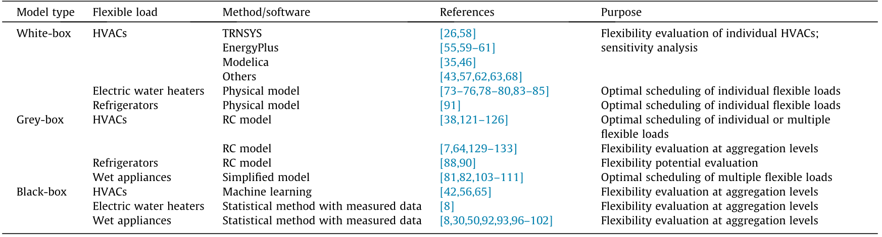
Table 8 summarizes the models employed in previous studies for different residential flexible loads. It can be seen that white-box models were widely adopted to model thermostatically controlled loads including HVACs, electric water heaters, and refrigerators. Various commercial software, including TRNSYS, EnergyPlus, and Modelica, were popular for evaluating the flexibility of individual HVACs and conducting parametric analyses. Simulations under different conditions such as various building envelopes, air conditioner terminals, climate zones, and demand-side management strategies can be easily realized with the help of commercial software. Hence, simulation software is suitable for quantifying the flexibility of individual HVACs. Moreover, white-box models have been employed in many studies [73–76,78-80,83–85] to optimize the scheduling of electric water heaters in order to provide flexibility and decrease electric bills, although only the flexibility of electric water heaters is considered in these papers. Grey-box models have mainly been applied to model HVACs and wet appliances, with sparse application to refrigerators. More specifically, RC models have usually been used to optimize the control of individual HVACs [123,124] or to optimize them together with other flexible loads [38,121,122,125,126]. These models have also been employed to evaluate the flexibility of HVACs at aggregation levels. In grey-box models of wet appliances, the actual wet appliance models are simplified into a set of sequential uninterruptible energy phases, in which the power is assumed to be constant in order to optimize the scheduling of the appliances. Black-box models have been widely deployed to model wet appliances, using statistical methods based on empirical data from pilot tests [127,128] to evaluate flexibility at aggregation levels. In addition, the load-shedding potential of HVACs at aggregation levels can be assessed with black-box models using machine learning approaches.
《Table 8》
Table 8 Summary of the models employed in previous studies on building demand flexibility.
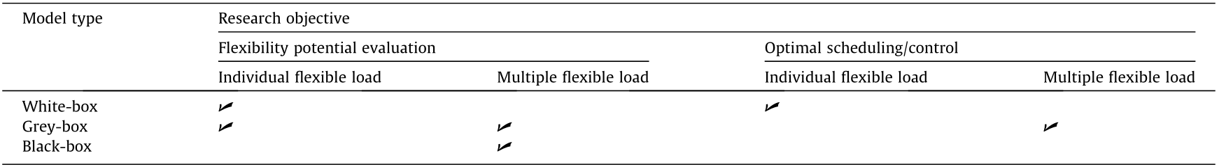
The above analysis shows that white-box models are considered much more when individual flexible loads are investigated. Grey-box models are mainly used to evaluate flexibility at aggregation levels and optimize scheduling with multiple flexible loads. Black-box models are adopted to quantify the flexibility at aggregation levels. Based on this analysis, Table 9 gives recommendations for model applications in diverse situations.
《Table 9》
Table 9 Recommendations for model applications under different conditions.
Although numerous studies have been conducted on modeling residential flexible loads, some challenges still exist. White-box models can describe the dynamic physical processes of flexible loads in detail. Nevertheless, they generally ignore the effects of household heterogeneity, occupant activities, and energy usage habits, especially when commercial software is deployed. In comparison, black-box models do not need complex physical models of household appliances and can directly quantify building demand flexibility based on behind-the-meter data with good accuracy and credibility, considering the occupants’ energy usage behavior. However, this approach requires large amounts of high-quality data, the acquisition of which is generally expensive and timeconsuming, as it may take several years. In addition, black-box models introduce concerns regarding the privacy of occupant information. An economic, effective, and precise way to acquire the actual load profile and usage patterns of household appliances is needed, preferably involving non-intrusive load monitoring [134] or a non-intrusive load-decomposition methodology [135]. Moreover, methods to model occupant behavior when interacting with smart appliances—which has a high level of uncertainty— are needed because of differences in building load types and discrepancies in the appliance usage habits of households. The factors of time, cost, and model accuracy must be comprehensively considered when a grey-box model is adopted. Models of residential flexible loads that incorporate appliances’ operation characteristics, energy usage patterns, and occupant behavior are needed.
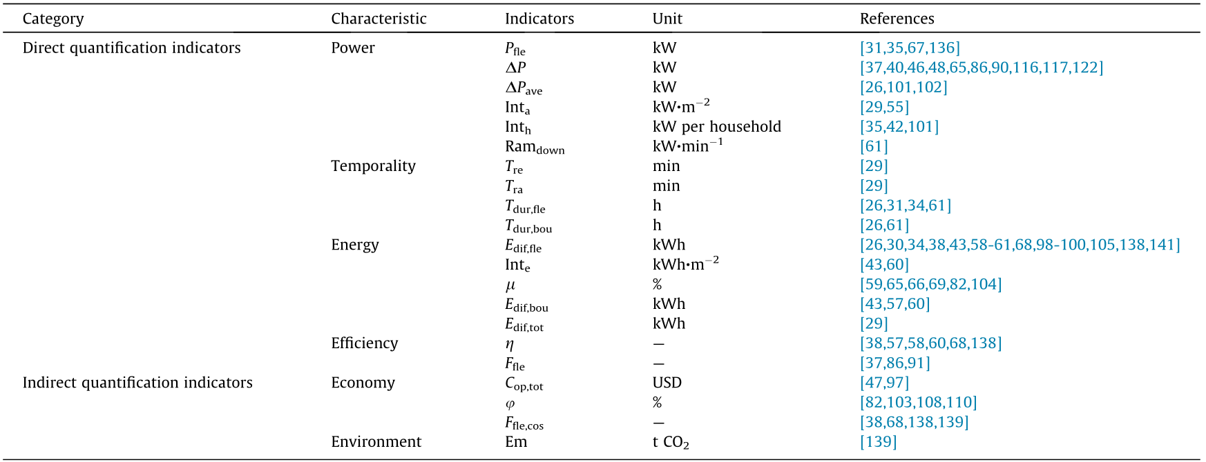
《6.2. Demand flexibility indicators》
6.2. Demand flexibility indicators
To quantify building demand flexibility, it is important to choose appropriate indicators that can characterize flexibility and demonstrate the benefits of flexibility from the viewpoint of different stakeholders. This section summarizes and categorizes flexibility evaluation metrics into direct and indirect quantification indicators. The former directly illustrate the features of building demand flexibility in various aspects, while indirect quantification indicators are related to the performance of buildings in regard to economic and environmental aspects.
6.2.1. Direct quantification indicators
Taking downward flexibility as an example, Fig. 8 presents a conceptual illustration of the response processes of a flexible load in a demand-response event. When a flexible load receives the activation signal, it takes some time to respond and takes actions to decrease power usage and operate for a period with minimum power. After the demand-response event ends, the flexible load takes some time to restore the appliance’s state to its original state. Various indicators have been used in previous studies to describe the characteristics of a flexible load during the different response processes of a demand-response event. The majority of previous studies have focused on the aspects of capacity, temporality, energy, and efficiency. More details are provided below.
《Fig. 8》
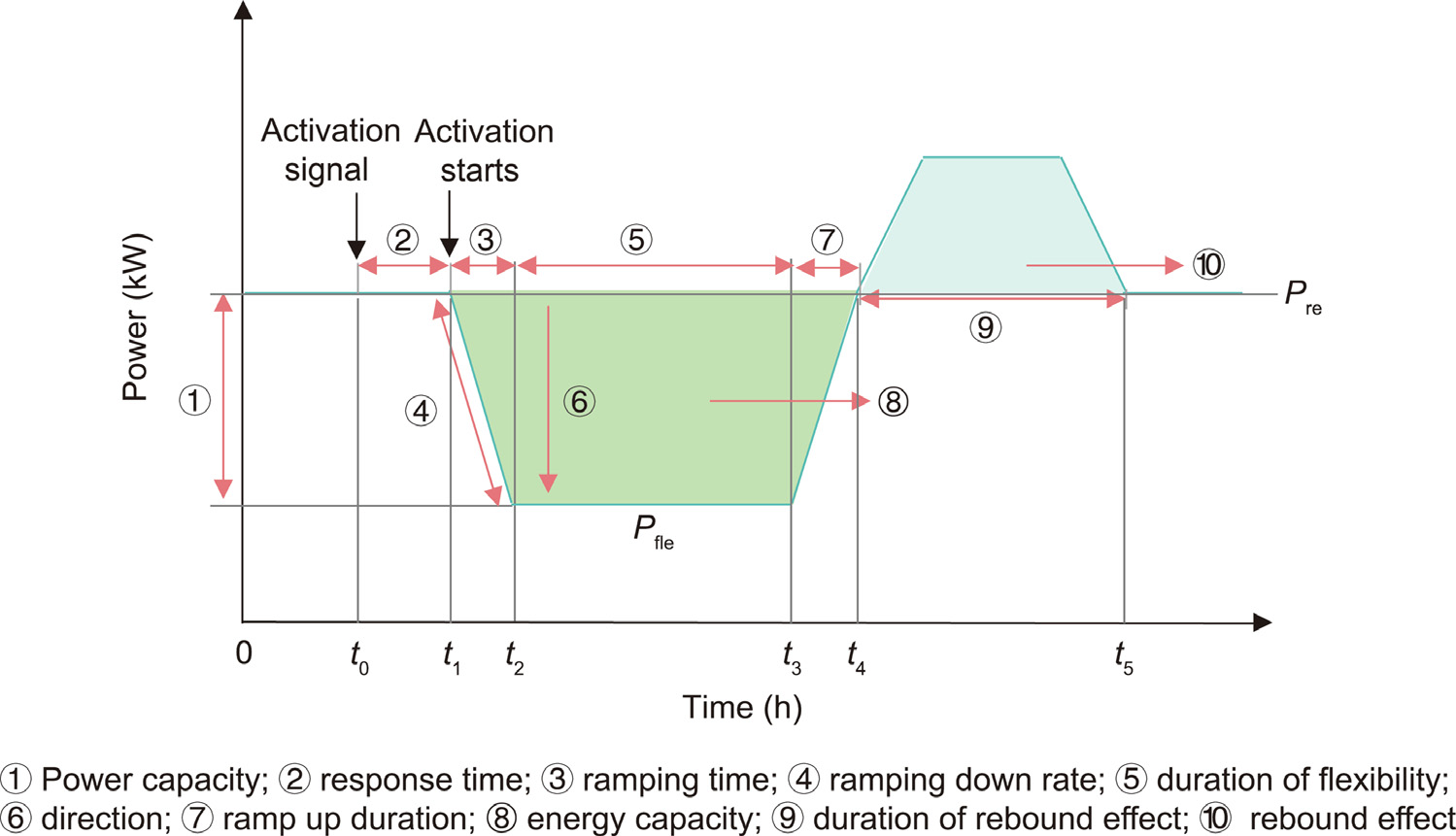
Fig. 8. Conceptual illustration of the response processes of a flexible load during a demand-response event. Pre is the power of the reference scenario; Pfle is the power during demand response.
Six indicators have been employed in the literature to evaluate the power properties of building demand flexibility. The power during demand response, Pfle, was adopted in Refs. [35,67,136]. Moreover, some studies [48,86] deployed the indicator  , which denotes the power differences during demand-response periods and can be calculated using Eq. (1). The average power difference during demand response,
  , was adopted in Ref. [26], and can be formulated with Eq. (2). In Ref. [29], the intensity of the power demand changes, Inta, which is defined as the average power demand changes during a response event normalized by the building floor area, was proposed, as presented in Eq. (3). Similar to the metric Inta, another indicator of power demand changes, Inth, was developed in Ref. [101], which is normalized by household and is expressed in Eq. (4). The normalization allows a comparison of these metrics across buildings with different sizes or types. In addition, the ramping-down rate, Ramdown, which is defined as the ratio of the time it takes for a flexible load to deliver its maximum flexibility to the maximum flexibility capacity,
  was employed in Refs. [29,61].
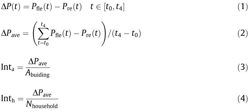

where, Pre is the power of the reference scenario, in which no response events are occurring; t0 and t4 are the start and end times of the response events, respectively; Abuilding is the area of the building floor; Nhousehold is the number of households; and t1 and t2 are the time the activation starts and the time at which the flexible load reaches its maximum flexibility.
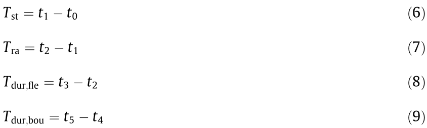
To investigate the temporality of building demand flexibility, the response time of a flexible load when a demand-response event takes places has been studied [19] and can be calculated using Eq. (6). The indicator, the response time Tst, refers to how fast the buildings respond to external signals, including electricity prices (κ(t)) and the fluctuation of distributed renewable energy generation. The ramping time, Tra, is ramping time that denotes the time it takes from the start of activation until the lowest/highest level is adopted [29] and can be calculated with Eq. (7). Researchers also care about how long the flexibility provided by buildings and the rebound effects caused by response events can last. The duration of a demand-response event,Tdur,fle, can be calculated using Eq. (8) [34,40], and the duration of the rebound effects, Tdur,bou, representing the time it takes to restore the nominal conditions is calculated using Eq. (9) [34].
As for the energy aspect of building demand flexibility, stakeholders have concentrated on energy-consumption reductions during demand-response periods, Edif,fle, and on the extra energy consumption in off-peak periods caused by rebound effects. The former is calculated by Eq. (10) [60]. The peak demand reduction intensity, Inte, and the peak demand reduction ratio, μ, have also been employed to describe the building’s energy-consumption changes, which can be calculated by Eqs. (11) and (12), respectively. Energy-consumption changes caused by rebound effects, Edif,bou, are expressed in Eq. (13) [47]. Another indicator, differences of energy consumption between demand response and rebound effects, Edif,tot, has also been used [29] and is shown in Eq. (14).
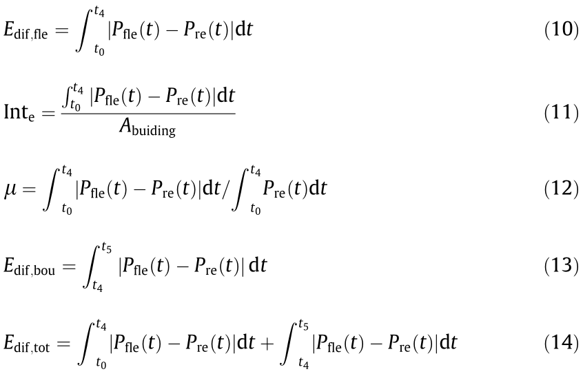
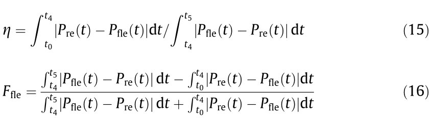
To provide demand flexibility, building owners must adjust their electricity-usage patterns, which results in changes to their total energy consumption. Hence, indicators have been proposed to describe these differences. Le Dreau et al. [60] developed the indicator of shedding or shifting efficiency, η, which refers to the capacity of available energy flexibility; it is defined as the ratio of energy consumption between the ‘‘rebound effect” and the ‘‘demand-response event,” which can be calculated by Eq. (15). According to this equation, the shift efficiency is a value from 0 to  in theory. Another indicator—the flexibility factor, Ffle—has been adopted in many studies and is expressed by Eq. (16). Ffle, ranges from –1 to 1 and is equal to 0 in the reference case [137,138].
6.2.2. Indirect quantification indicators
Apart from metrics that directly characterize building demand flexibility, indirect quantification indicators are also employed to evaluate the economic and environmental performance for a demand-response event. Building owners mainly focus on the economic benefits when providing flexibility, while governments and society care more about CO2 emissions reduction and utility grid stability, especially in the context of pursuing carbon neutrality. The impact of building demand flexibility on economic cost and carbon reduction is integrated. Building demand flexibility can reduce the operating cost and CO2 emissions when peak shaving, but the rebound effect will increase the cost and emissions. Hence, economic and environmental benefits are usually considered over the duration of a demand-response event and rebound effect, as represented by Eqs. (17)–(20).
Operation costs saving, Cop,tot, and operation costs reduction ratio, φ, respectively calculated by Eqs. (17) and (18), are usually chosen to assess the economic benefits of demand flexibility. Moreover, similar to the concept of flexibility factor, the cost flexibility factor, Ffle,cos, has been used in Refs. [42,77,121]. The Ffle,cos is expressed by Eq. (19), where κ(t) is the electricity price. As for the environmental performance evaluation, an indicator of CO2 emission reductions, Em, has been used and can be calculated by Eq. (20) [139], where  represents the equivalent emissions coefficient of the energy imported from the utility grid.

6.2.3. Summary of demand flexibility evaluation indicators
Numerous static evaluation indicators for demand flexibility have been proposed in previous studies, referring to power, temporality, energy, efficiency, economic, and environmental aspects. A summary of the demand flexibility indicators introduced in Section 6.2 is presented in Table 10. It can be seen that different metrics have been employed to quantify residential building demand flexibility. The wide range of different indicators stems from the fact that there are no commonly accepted definitions in relation to building demand flexibility [20]. It is also caused by the fact that building demand flexibility involves several stakeholders with different perspectives and targets, which are dependent on the specific services enabled. Several indicators that are relevant to various stakeholders were developed to quantify building demand flexibility by Zhang et al. [140]. Table 10 also shows that two metrics,  , and Edif,fle have been used more frequently than the other indicators. Six indicators— namely, Pfle, Tdur,fle, μ, η, φ, and Ffle,cos—have been employed in several studies. The remaining indicators presented in Table 10 are rarely used. This fact also backs up the viewpoint presented in Section 5.6: that there is a lack of studies on the response characteristics of different flexible loads. Many of the metrics included in this table to describe the response characteristics of flexible loads have rarely been used. Except for the first two indicators in Table 10, the other metrics are static, and cannot represent the availability of flexibility because building demand flexibility strongly depends on the initial boundary conditions and time of the day. Moreover, these indicators were proposed for quantifying the flexibility of HVACs and wet appliances at the device level. Thus, they may be not applicable at the building level, where various flexible loads on the building demand side are aggregated together.
《Table 10》
Table 10 Summary of indicators employed to quantify building demand flexibility in previous studies.
It is difficult to compare the flexibility potential evaluated across different studies, even for the same flexible load, due to the lack of uniform evaluation indicators. Formulating a comprehensive metric to quantify building demand flexibility may be challenging, due to the diverse nature of such flexibility. Nevertheless, a systematic evaluation framework to quantify the flexibility potential of diverse flexible loads at different spatial scales with corresponding indicators is feasible. There is an urgent need for this consensus and standardized evaluation framework. Furthermore, easy-to-use and scalable tools facilitating the assessment of building demand flexibility and the provision of grid services need to be developed in the future.
《7. Conclusions》
7. Conclusions
This paper reviewed recent studies on the demand flexibility of residential buildings in regard to definitions, flexible loads, and quantification methods. Several terms associated with the flexibility of buildings, including energy flexibility, demand flexibility, load flexibility, and operation flexibility, were distinguished. Various definitions related to building demand flexibility were compared and analyzed, and a comprehensive definition was proposed. Then, the flexibility capabilities and operation characteristics of the main residential flexible loads were summarized and discussed. In addition, the models and evaluation indicators used to quantify residential building demand flexibility were classified into different categories and summarized. Based on a comprehensive literature review, research gaps, challenges, and potential future developments were pointed out. The main outcomes of the literature review are summarized as follows:
• There is no commonly accepted definition or uniform understanding of building demand flexibility. A more comprehensive definition was proposed in this study. Building demand flexibility is defined as the ability to manage a building’s flexible resources in order to change its load profile to meet different requirements without sacrificing end-user interests.
• Various residential flexible loads have different flexibility capabilities and operation characteristics to provide utility grid services. Thermostatically controlled loads can be shed, shifted, and modulated; lighting loads can not only be shed but also be modulated; and wet appliances only provide load-shifting services. These appliances have different running modes, usage frequencies, and seasonal features. However, a detailed analysis of the operation characteristics of these flexible loads, such as the power features at different operation stages, should be conducted based on the actual appliances’ operation data. Moreover, it is urgent to explore the response characteristics of these flexible loads, such as response speed, ramping duration, services duration, energy shifting, or shedding potential.
• Recommendations for the applications of models to different situations have been provided. White-box models are best suited to evaluate the building demand flexibility and optimize scheduling when individual flexible loads are considered; grey-box models are suitable for flexibility quantification at aggregation levels and to optimize scheduling with multiple flexible loads; and black-box models are more suitable for assessing the flexibility potential at aggregated levels. There is also a need to establish models of residential flexible loads that incorporate the appliances’ operation characteristics, energy usage patterns, and occupant behavior.
• A great deal of static demand flexibility evaluation indicators for power, temporality, energy, efficiency, economic, and environmental aspects have been proposed in previous publications. Nevertheless, a consensus and standardized evaluation framework to quantify residential building demand flexibility is lacking. Special efforts should be dedicated to the framework in order to quantify residential demand flexibility, considering the response characteristics of various flexible loads and the benefits to different stakeholders. Moreover, easy-to-use and scalable tools facilitating the assessment of building demand flexibility and the provision of grid services must be developed in the future.
《Acknowledgments》
Acknowledgments
The authors gratefully acknowledge the financial support of the Science and Technology Innovation Program of Hunan Province (2020RC5003), the research and application of key technologies for zero-energy buildings based on distributed energy storage and air conditioning demand response (2020-K-165), the Technology Innovation Program of Hunan Province (2017XK2015), and the Technology Innovation Program of Hunan Province (2020RC2017).
《Compliance with ethics guidelines》
Compliance with ethics guidelines
Zhengyi Luo, Jinqing Peng, Jingyu Cao, Rongxin Yin, Bin Zou, Yutong Tan, and Jinyue Yan declare that they have no conflict of interest or financial conflicts to disclose.


 京公网安备 11010502051620号


